MPAS Mesh Specification

Summary

This document describes the required fields for an MPAS mesh. In addition, it defines required orderings when creating an MPAS mesh. These together fully describe the MPAS mesh type and allow users to more easily understand what makes an MPAS mesh.

The vertical coordinate and related variables and attributes are added after mesh creation and are not addressed in this document.

Definitions and conventions

The meshes used by MPAS are Voronoi tessellations (VTs), in which MPAS identifies three types of elements: cells, edges, and vertices. Cells are simply the Voronoi cells in the tessellation, edges are the boundaries between adjacent Voronoi cells, and vertices are the corners of cells. In MPAS, cells are nominally located at the Voronoi generating points, which, for centroidal Voronoi tessellations, are the mass centroids of the Voronoi cells with respect to a density function, and edges are nominally located at the midpoints of edges. Fig. 1 shows three cells with their associated edges and vertices.

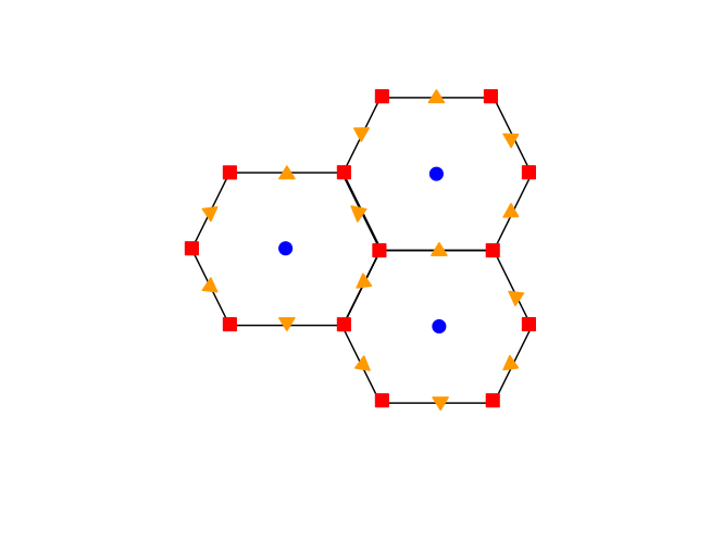
Fig. 1 Three cell Voronoi tessellation with cells denoted by blue circles, edges by orange triangles, and vertices by red squares.

The VT meshes used by MPAS may be defined on the Cartesian plane or on a sphere. In the case of planar meshes, areas and distances are assumed to be Euclidean, and the mesh is defined on the plane \(z = 0\). On a planar mesh, eastward is the \(x\) direction and northward is the \(y\) direction.

In the case of spherical meshes, areas and distances are computed in spherical geometry; cells, edges, and vertices are constrained to lie on the surface of the sphere, and the sphere is centered at the origin, \((x,y,z) = (0,0,0)\). In all cases, the coordinate systems assumed by MPAS meshes are right-handed. Fig. 2 illustrates VT meshes on the Cartesian plane and on the sphere. There are no requirements for the radius of the sphere, however an attribute sphere_radius is required that defines the radius of the sphere.

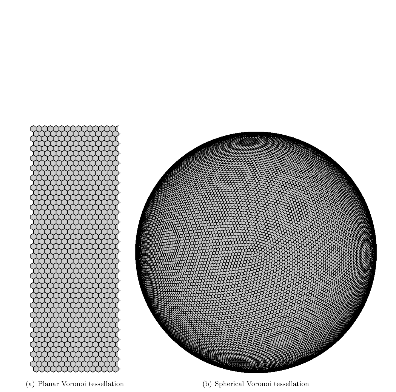
Fig. 2 Examples of Voronoi tessellations.

Grid description

The MPAS grid system requires the definition of seven elements. These seven elements are composed of two types of cells, two types of lines, and three types of points. These elements are depicted in Fig. 3 and defined in Table 1. These elements can be defined on either the plane or the surface of the sphere. The two types of cells form two meshes, a primal mesh composed of Voronoi regions and a dual mesh composed of Delaunay triangles. Each corner of a primal mesh cell is uniquely associated with the “center” of a dual mesh cell and vice versa. So we define the two mesh as either a primal mesh (composed of cells \(P_i\)) or a dual mesh (composed of cells \(D_v\)). The center of any primal mesh cell, \(P_i\), is denoted by \({\bf x}_i\) and the center of any dual mesh cell, \(D_v\), is denoted by \({\bf x}_v\). The boundary of a given primal mesh cell \(P_i\) is composed of the set of lines that connect the \({\bf x}_v\) locations of associated dual mesh cells \(D_v\). Similarly, the boundary of a given dual mesh cell \(D_v\) is composed of the set of lines that connect the \({\bf x}_i\) locations of the associated primal mesh cells \(P_i\).

As shown in Fig. 3, a line segment that connects two primal mesh cell centers is uniquely associated with a line segment that connects two dual mesh cell centers. We assume that these two line segments cross and the point of intersection is labeled as \({\bf x}_e\). In addition, we assume that these two line segments are orthogonal as indicated in Fig. 3. Each \({\bf x}_e\) is associated with two distances: \(d_e\) measures the distance between the primal mesh cells sharing \({\bf x}_e\) and \(l_e\) measures the distance between the dual mesh cells sharing \({\bf x}_e\).

Since the two line segments crossing at \({\bf x}_e\) are orthogonal, these line segments form a convenient local coordinate system for each edge. At each \({\bf x}_e\) location a unit vector \({\bf n}_e\) is defined to be parallel to the line connecting primal mesh cells. A second unit vector \({\bf t}_e\) is defined such that \({\bf t}_e = {\bf k} \times {\bf n}_e\).

In addition to these seven element types, we require the definition of sets of elements. In all, eight different types of sets are required and these are defined and explained in Table 2 and Fig. 4. The notation is always of the form of, for example, \(i \in CE(e)\), where the LHS indicates the type of element to be gathered (cells) based on the RHS relation to another type of element (edges).

Table 3 provides the names of all elements and all sets of elements as used in the MPAS framework. Elements appear twice in the table when described in the grid file in more than one way, e.g. points are described with both Cartesian and latitude/longitude coordinates.

An ncdump -h of an MPAS mesh, output, or restart file should contain the mesh-variable names listed in Table 3.

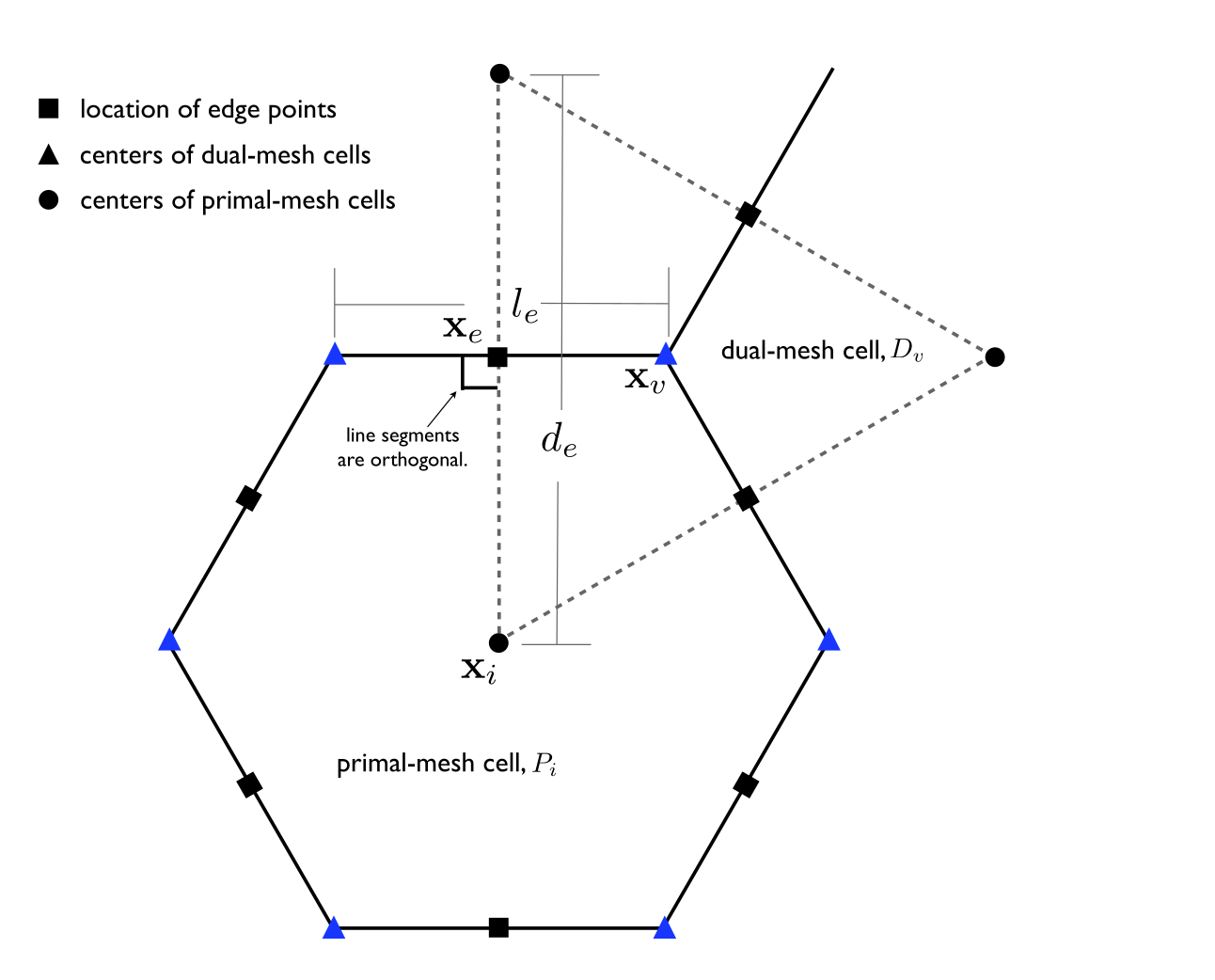
Fig. 3 Definition of elements used to build the MPAS grid. Also see Table 1.

Table 1 Definition of elements used to build the MPAS grid.

Element	Type	Definition
\({\bf x}_i\)	point	location of center of primal-mesh cells
\({\bf x}_v\)	point	location of center of dual-mesh cells
\({\bf x}_e\)	point	location of edge points where velocity is defined
\(d_e\)	line segment	distance between neighboring \({\bf x}_i\) locations
\(l_e\)	line segment	distance between neighboring \({\bf x}_v\) locations
\(P_i\)	cell	a cell on the primal-mesh
\(D_v\)	cell	a cell on the dual-mesh

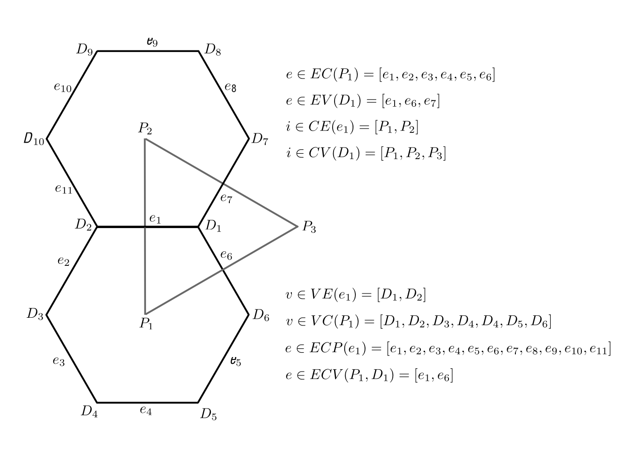
Fig. 4 Definition of element groups used to reference connections in the MPAS grid. Also see Table 2.

Table 2 Definition of element groups used to reference connections in the MPAS grid.

Syntax	Output
\(e \in EC(i)\)	set of edges that define the boundary of \(P_i\).
\(e \in EV(v)\)	set of edges that define the boundary of \(D_v\).
\(i \in CE(e)\)	two primal-mesh cells that share edge \(e\).
\(i \in CV(v)\)	set of primal-mesh cells that form the vertices of dual mesh cell \(D_v\).
\(v \in VE(e)\)	the two dual-mesh cells that share edge \(e\).
\(v \in VI(i)\)	the set of dual-mesh cells that form the vertices of primal-mesh cell \(P_i\).
\(e \in ECP(e)\)	edges of cell pair meeting at edge \(e\).
\(e \in EVC(v,i)\)	edge pair associated with vertex \(v\) and mesh cell \(i\).

Table 3 Variable names used to describe an MPAS grid.

Element	Name	Size	Comment
\({\bf x}_i\)	{x,y,z}Cell	nCells	Cartesian location of \({\bf x}_i\)
\({\bf x}_i\)	{lon,lat}Cell	nCells	longitude and latitude of \({\bf x}_i\)
\({\bf x}_v\)	{x,y,z}Vertex	nVertices	Cartesian location of \({\bf x}_v\)
\({\bf x}_v\)	{lon,lat}Vertex	nVertices	longitude and latitude of \({\bf x}_v\)
\({\bf x}_e\)	{x,y,z}Edge	nEdges	Cartesian location of \({\bf x}_e\)
\({\bf x}_e\)	{lon,lat}Edge	nEdges	longitude and latitude of \({\bf x}_e\)
\(d_e\)	dcEdge	nEdges	distance between \({\bf x}_i\) locations
\(l_e\)	dvEdge	nEdges	distance between \({\bf x}_v\) locations
\(e \in EC(i)\)	edgesOnCell	(maxEdges, nCells)	edges that define \(P_i\)
\(e \in EV(v)\)	edgesOnVertex	(vertexDegree, nVertices)	edges that define \(D_v\)
\(i \in CE(e)\)	cellsOnEdge	(2, nEdges)	primal-mesh cells that share edge \(e\)
\(i \in CV(v)\)	cellsOnVertex	(vertexDegree, nVertices)	primal-mesh cells that define \(D_v\)
\(v \in VE(e)\)	verticesOnEdge	(2, nEdges)	dual-mesh cells that share edge \(e\)
\(v \in VI(i)\)	verticesOnCell	(maxEdges, nCells)	vertices that define \(P_i\)

Grid dimensions

Dimension	Description
Time	netCDF record (unlimited) dimension
nCells	Number of cells in the grid
nEdges	Number of edges (cell faces) in the grid
nVertices	Number of vertices (cell corners) in the grid
maxEdges	Maximum number of edges on any cell, equal to max neigbor cells
maxEdges2	Twice maxEdges
vertexDegree	Number of edges incident with each vertex (3 for Delaunay dual grid)
TWO	Constant value 2
THREE	Constant value 3
FIFTEEN	Constant value 15
TWENTYONE	Constant value 21
R3	Constant value 3
StrLen	Length of strings

Horizontal mesh fields

The Read by column indicates how Omega obtains each field:

• HorzMeshIn — read from the mesh file by the HorzMeshIn I/O stream and field group, which are defined by the HorzMesh class.

• Decomp — read and redistributed by the Decomp class before HorzMesh is constructed. These arrays hold local addresses that depend on the domain decomposition, so they are neither read nor written by HorzMesh.

• — — not read by Omega.

Field	Read by	Description
double latCell(nCells)	HorzMeshIn	Cell center latitude (rad)
double lonCell(nCells)	HorzMeshIn	Cell center longitude (rad)
double xCell(nCells)	HorzMeshIn	Cell center x-coordinate (m; scaled by sphere_radius on a sphere)
double yCell(nCells)	HorzMeshIn	Cell center y-coordinate (m; scaled by sphere_radius on a sphere)
double zCell(nCells)	HorzMeshIn	Cell center z-coordinate (m; scaled by sphere_radius on a sphere)
int indexToCellID(nCells)	Decomp	Global cell ID
double latEdge(nEdges)	HorzMeshIn	Edge latitude (rad)
double lonEdge(nEdges)	HorzMeshIn	Edge longitude (rad)
double xEdge(nEdges)	HorzMeshIn	Edge x-coordinate (m; scaled by sphere_radius on a sphere)
double yEdge(nEdges)	HorzMeshIn	Edge y-coordinate (m; scaled by sphere_radius on a sphere)
double zEdge(nEdges)	HorzMeshIn	Edge z-coordinate (m; scaled by sphere_radius on a sphere)
int indexToEdgeID(nEdges)	Decomp	Global edge ID
double latVertex(nVertices)	HorzMeshIn	Vertex latitude (rad)
double lonVertex(nVertices)	HorzMeshIn	Vertex longitude (rad)
double xVertex(nVertices)	HorzMeshIn	Vertex x-coordinate (m; scaled by sphere_radius on a sphere)
double yVertex(nVertices)	HorzMeshIn	Vertex y-coordinate (m; scaled by sphere_radius on a sphere)
double zVertex(nVertices)	HorzMeshIn	Vertex z-coordinate (m; scaled by sphere_radius on a sphere)
int indexToVertexID(nVertices)	Decomp	Global vertex ID
int cellsOnEdge(nEdges, TWO)	Decomp	IDs of the two cells separated by each edge
int nEdgesOnCell(nCells)	Decomp	Number of edges forming the border of each cell
int nEdgesOnEdge(nEdges)	Decomp	Number of edges used in computing tangential velocity for each edge
int edgesOnCell(nCells, maxEdges)	Decomp	IDs of edges forming boundary of each cell
int edgesOnEdge(nEdges, maxEdges2)	Decomp	IDs of edges used in computing tangential velocity for each edge
double weightsOnEdge(nEdges, maxEdges2)	HorzMeshIn	Weights used in computing tangential velocity for each edge; could be computed internally
double dvEdge(nEdges)	HorzMeshIn	Distance (in spherical geometry) between end points of each edge; could be computed internally
double dcEdge(nEdges)	HorzMeshIn	Distance (in spherical geometry) between cell centers separated by each edge; could be computed internally
double angleEdge(nEdges)	HorzMeshIn	Angle between positive normal direction and local east vector for each edge, as illustrated in Fig. 5; could be computed internally
double areaCell(nCells)	HorzMeshIn	Area (in spherical geometry) of each cell, or -1 for an incomplete cell; could be computed internally
double areaTriangle(nVertices)	HorzMeshIn	Area (in spherical geometry) of each dual-grid cell (Delaunay triangle); could be computed internally
int cellsOnCell(nCells, maxEdges)	Decomp	IDs of neighbor cells for each cell
int verticesOnCell(nCells, maxEdges)	Decomp	IDs of corner points (vertices) for each cell
int verticesOnEdge(nEdges, TWO)	Decomp	IDs of vertices forming endpoints for each edge
int edgesOnVertex(nVertices, vertexDegree)	Decomp	IDs of edges incident with each vertex
int cellsOnVertex(nVertices, vertexDegree)	Decomp	IDs of cells that meet at each vertex
double kiteAreasOnVertex(nVertices, vertexDegree)	HorzMeshIn	Areas (in spherical geometry) of intersections between primal- and dual-grid cells; could be computed internally
double meshDensity(nCells)	HorzMeshIn	SCVT density function evaluated at cell centers; read from the mesh generator input rather than computed

Coordinate-value conventions

The latitude and longitude fields use radians and follow these value conventions:

Fields	Valid values or convention
latCell, latEdge, latVertex	\(-\pi/2 \leq \mathrm{latitude} \leq \pi/2\)
lonCell, lonEdge, lonVertex	\(0 \leq \mathrm{longitude} \leq 2\pi\)
All latitude and longitude fields on a planar mesh	Constant value of 0

Edge angles

angleEdge may be defined equivalently as the angle that the positive normal direction \(\vec{u}\) makes with the local eastward direction (shown in Definition of angleEdge, the angle between the positive normal direction \vec{u} and the local eastward direction. Equivalently, it is the angle), or as the angle that the positive tangential direction \(\vec{v}\) makes with the local northward direction.

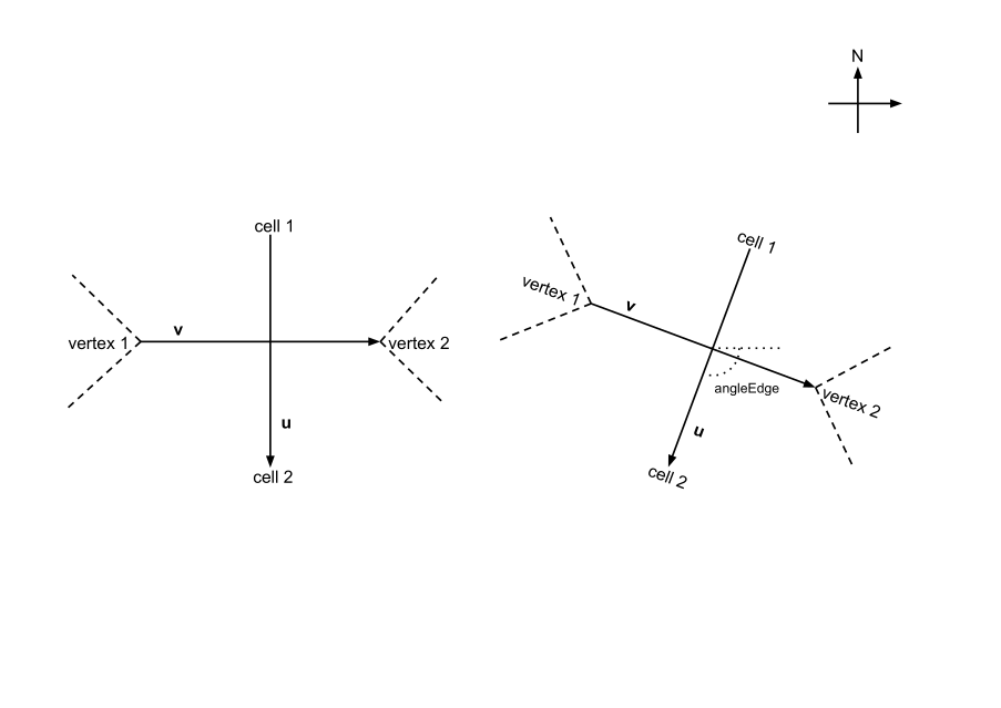
Fig. 5 Definition of angleEdge, the angle between the positive normal direction \(\vec{u}\) and the local eastward direction. Equivalently, it is the angle

Reference formulations

Two equivalent formulations are used in practice. Both satisfy the definition above, but the former was found to be more accurate on spherical meshes.

Normal-and-east formulation

Let \(\hat{\mathbf{e}}\) and \(\hat{\mathbf{n}}\) be the local eastward and northward unit vectors at \({\bf x}_e\),

\[ \hat{\mathbf{e}} = \frac{\hat{\mathbf{k}} \times {\bf x}_e}{\|\hat{\mathbf{k}} \times {\bf x}_e\|}, \qquad \hat{\mathbf{n}} = \frac{{\bf x}_e \times \hat{\mathbf{e}}}{\|{\bf x}_e \times \hat{\mathbf{e}}\|}, \]

where \(\hat{\mathbf{k}}\) is the Cartesian \(z\) axis. The edge-normal direction is recovered from the tangential vector as \(\vec{u} \propto \vec{v} \times {\bf x}_e\), and its eastward and northward components are

\[ u_e = \left(\vec{v} \times {\bf x}_e\right) \cdot \hat{\mathbf{e}}, \qquad u_n = \left(\vec{v} \times {\bf x}_e\right) \cdot \hat{\mathbf{n}}. \]

The angle then follows directly from a two-argument arctangent,

\[ \mathrm{angleEdge} = \mathrm{atan2}\left(u_n,\, u_e\right), \]

which returns a value in \((-\pi, \pi]\). This formulation is used by the Polaris spherical base-mesh step.

Tangential-and-north formulation

Equivalently, the angle may be obtained from the change in latitude along the edge. On the unit sphere,

\[ \alpha = \arccos\left( \mathrm{clamp}\left( \frac{\mathrm{lat}_{v_2} - \mathrm{lat}_{v_1}}{l_e},\, -1,\, 1 \right)\right), \]

where \(l_e\) is dvEdge expressed on the unit sphere, that is, dvEdge divided by sphere_radius. Because \(\arccos\) is even, this yields only the magnitude of the angle; the sign is taken from the orientation of \(\mathbf{x}_{v_2}\) relative to a reference point displaced slightly northward from \({\bf x}_e\), and the result is then wrapped into \([-\pi, \pi]\),

\[ \mathrm{angleEdge} = \left(s\,\alpha + \pi \bmod 2\pi\right) - \pi, \qquad s = \pm 1 . \]

This formulation is used by MpasMeshConverter.x.

On a planar mesh, both formulations reduce to the angle between the edge-normal vector and the \(x\) axis,

\[\begin{split} \mathrm{angleEdge} = \begin{cases} \theta, & u_y \geq 0 \\ 2\pi - \theta, & u_y < 0 \end{cases} \qquad \theta = \arccos\left(\frac{u_x}{\|\vec{u}\|}\right), \end{split}\]

with \(\vec{u}\) evaluated after any periodic adjustment of \(\mathbf{x}_{\mathrm{cellsOnEdge}(2,\mathrm{iEdge})}\) relative to \(\mathbf{x}_{\mathrm{cellsOnEdge}(1,\mathrm{iEdge})}\).

Recovering earth-relative vectors

Given a vector \((u_\perp, u_\parallel)\) defined in terms of components orthogonal to and parallel to the edge, the earth-relative components \((u,v)\) in the local eastward and northward directions are

\[\begin{split} \begin{bmatrix} u \\ v \\ \end{bmatrix} = \begin{bmatrix} \cos\alpha & -\sin\alpha \\ \sin\alpha & \cos\alpha \\ \end{bmatrix} \begin{bmatrix} u_\perp \\ u_\parallel \\ \end{bmatrix}, \end{split}\]

where \(\alpha = {\rm angleEdge}\). This relation holds for either reference formulation, since it depends on \(\alpha\) only through \(\cos\alpha\) and \(\sin\alpha\).

Global attributes

The following global attributes are required by the MPAS framework. All MPAS meshes should contain these global attributes.

Attribute	Type	Valid values	Description
on_a_sphere	character	"YES" or "NO"	Defines whether the mesh describes points that lie on the surface of a sphere.
sphere_radius	double	any non-negative real value	Radius of the sphere the points are defined on. Set to 0 for a planar mesh.
is_periodic	character	"YES" or "NO"	Defines whether the mesh has any periodic boundaries. Only meaningful when on_a_sphere is "NO".
mesh_spec	character	any valid version of the MPAS mesh specification	Version of the MPAS mesh specification the mesh conforms to.
file_id	character	any combination of lowercase letters and numbers	Random string used for tracking mesh provenance.
parent_id	character	one or more file_id values, newline separated	Provenance chain of the files this mesh was derived from.
Conventions	character	"MPAS"	Identifies the file as following MPAS conventions.
source	character	name of the generating tool	Tool that produced the mesh, e.g. MpasMeshConverter.x.
history	character	free text	Command line used to produce the mesh, prepended to any inherited history.

When is_periodic is set to "YES", the following two attributes are required as well:

Attribute	Type	Valid values	Description
x_period	double	any positive real value	Period of the mesh in the \(x\) direction.
y_period	double	any positive real value	Period of the mesh in the \(y\) direction.

Connectivity and ordering requirements

Connectivity arrays that describe corresponding elements must use consistent ordering. For example, edgesOnCell(n, iCell) must identify the edge between iCell and cellsOnCell(n, iCell).

When creating an MPAS mesh, it is recommended to establish connectivity and ordering relative to edges first, then vertices, and finally cells.

Missing values and padding

A mesh may contain a cell with no neighbor across one or more edges, such as an ocean mesh from which land cells have been removed. In this case, the missing entry in a connectivity array such as cellsOnCell must be represented by 0.

Connectivity arrays also need padding when an element has fewer entries than the corresponding maximum dimension. For example, if a mesh contains a heptagon, maxEdges is 7, while hexagons and pentagons have only 6 and 5 valid entries. MPAS itself does not prescribe the padding values, and reference mesh generation tools pad with zeros. Some external tools instead require repetition of the final valid entry. Use a convention that is consistent across the complete tool chain.

Requirements relative to edges

The edge-normal and tangential vectors and the angleEdge convention are defined in Edge angles. In addition, the edge connectivity arrays must satisfy the following ordering requirements:

• edgesOnEdge must proceed counter-clockwise, beginning with the edges that surround cellsOnEdge(1, iEdge) and ending with the edges that surround cellsOnEdge(2, iEdge).

• The current edge is omitted from edgesOnEdge, but it may be treated as both the starting and ending location when checking counter-clockwise ordering.

• weightsOnEdge must use exactly the same ordering as edgesOnEdge; thus, weightsOnEdge(n, iEdge) applies to edgesOnEdge(n, iEdge). The weights are those of the TRiSK formulation of Thuburn et al., J. Comput. Phys., 2009, and depend on dcEdge, dvEdge, areaCell, and kiteAreasOnVertex.

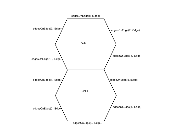
Fig. 6 Counter-clockwise ordering of edgesOnEdge around the two cells that share an edge.

Requirements relative to vertices

• cellsOnVertex and edgesOnVertex must proceed counter-clockwise around a vertex.

• Cells and edges alternate around a vertex, with cellsOnVertex(n, iVertex) lying counter-clockwise of edgesOnVertex(n, iVertex) and clockwise of edgesOnVertex(n+1, iVertex). For every valid \(n\), the vector

  \[ \left(\mathbf{x}_{\mathrm{edgesOnVertex}(n,\mathrm{iVertex})} - \mathbf{x}_{\mathrm{iVertex}}\right) \times \left(\mathbf{x}_{\mathrm{cellsOnVertex}(n,\mathrm{iVertex})} - \mathbf{x}_{\mathrm{iVertex}}\right) \]

  must point in the local outward-normal direction. The indices in this expression represent their corresponding Cartesian position vectors.

  This has the same sense as the corresponding requirement relative to cells below, where verticesOnCell(n, iCell) likewise lies counter-clockwise of edgesOnCell(n, iCell).

• kiteAreasOnVertex(n, iVertex) is the intersection of areaTriangle(iVertex) with areaCell(cellsOnVertex(n, iVertex)). It follows from the ordering above that this kite is the quadrilateral bounded by iVertex, edgesOnVertex(n, iVertex), cellsOnVertex(n, iVertex), and edgesOnVertex(n+1, iVertex), where the edge index wraps back to 1 for the last kite.

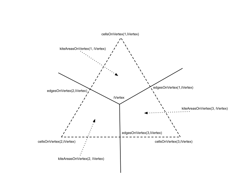
Fig. 7 Ordering of cells, edges, and kite areas relative to a vertex.

Requirements relative to cells

• cellsOnCell, edgesOnCell, and verticesOnCell must each proceed counter-clockwise around a cell.

• edgesOnCell(n, iCell) must be the edge between iCell and cellsOnCell(n, iCell).

• verticesOnCell(n, iCell) must lead both edgesOnCell(n, iCell) and cellsOnCell(n, iCell). For every valid \(n\), the vector

  \[ \left(\mathbf{x}_{\mathrm{edgesOnCell}(n,\mathrm{iCell})} - \mathbf{x}_{\mathrm{iCell}}\right) \times \left(\mathbf{x}_{\mathrm{verticesOnCell}(n,\mathrm{iCell})} - \mathbf{x}_{\mathrm{iCell}}\right) \]

  must point in the local outward-normal direction. The same requirement holds when cellsOnCell is substituted for edgesOnCell. The indices in these expressions represent their corresponding Cartesian position vectors.

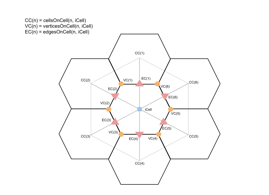
Fig. 8 Consistent counter-clockwise ordering of cells, edges, and vertices relative to a cell.

Boundary representation

Some meshes need to represent boundaries between active and inactive regions, between ocean and land, or between a nested mesh and its parent mesh. A boundary edge is represented through cellsOnEdge: when the second entry, cellsOnEdge(2, iEdge), is 0, the edge is treated as a boundary edge.

Optional and diagnostic fields

The following fields are not required by this specification. Some are written by mesh-generation tools as diagnostics, and others are commonly computed internally by MPAS cores.

Field	Read by	Description
int boundaryVertex(nVertices)	—	1 if the vertex has fewer than vertexDegree valid cells, 0 otherwise
double cellQuality(nCells)	—	Ratio of the minimum to maximum dvEdge on each cell
double gridSpacing(nCells)	—	Mean dcEdge over the edges of each cell
double triangleQuality(nVertices)	—	Ratio of the minimum to maximum dcEdge on each dual cell
double triangleAngleQuality(nVertices)	—	Ratio of the minimum to maximum interior angle of each dual triangle
int obtuseTriangle(nVertices)	—	1 if the dual triangle contains an obtuse angle, 0 otherwise
double edgeNormalVectors(nEdges, R3)	—	Vectors in Cartesian space normal to each edge
double localVerticalUnitVectors(nCells, R3)	—	Vectors in Cartesian space pointing in the local vertical direction at cell centers
double cellTangentPlane(nCells, TWO, R3)	—	Two orthonormal vectors in the tangent plane of each cell
double fCell(nCells)	HorzMeshIn	Coriolis parameter at cell centers (radians s^-1)
double fEdge(nEdges)	HorzMeshIn	Coriolis parameter at edges (radians s^-1)
double fVertex(nVertices)	HorzMeshIn	Coriolis parameter at vertices (radians s^-1)