Tendency Terms

Tendencies for updating state variables are computed using functors, which are class objects that can be called like functions. These functors are used within Kokkos parallel loops to compute the full tendency arrays. The following tendency terms are currently implemented:

Name	Description
PseudoThicknessFluxDivOnCell	divergence of pseudo-pseudo-thickness flux, defined at cell center
PotentialVortHAdvOnEdge	horizontal advection of potential vorticity, defined on edges
KEGradOnEdge	gradient of kinetic energy, defined on edges
SSHGradOnEdge	gradient of sea-surface height, multiplied by gravitational acceleration, defined on edges
VelocityDiffusionOnEdge	Laplacian horizontal mixing, defined on edges
VelocityHyperDiffOnEdge	biharmonic horizontal mixing, defined on edges
TracerHorzAdvOnCell	horizontal advection of thickness-weighted tracers
TracerDiffOnCell	horizontal diffusion of thickness-weighted tracers
TracerHyperDiffOnCell	biharmonic horizontal mixing of thickness-weighted tracers
SfcStressForcingOnEdge	forcing by surface stress (e.g. wind), defined on edges
BottomDragOnEdge	bottom drag, defined on edges
SfcThicknessForcingOnCell	surface pseudo-thickness forcing from coupled freshwater and salt fluxes, defined on cells
SfcTracerForcingOnCell	surface tracer forcing from coupled heat and salt fluxes, with direct heat always and mass-flux enthalpy terms gated by thickness forcing, defined on cells
PenetratingShortwaveOnCell	depth-dependent three-band shortwave heating, defined on cells
SurfaceTracerRestoringOnCell	surface tracer restoring, defined on cells

Among the internal data stored by each functor is a bool which can enable or disable the contribution of that particular term to the tendency. These flags need to be provided in the configuration file:

Tendencies:
   ThicknessFluxTendencyEnable: true

Some functors have member variables that can be set by the user by the configuration file. The following are all the user-configurable parameters for the currently available tendency terms:

Term	Parameter	Description
PseudoThicknessFluxDivOnCell	ThicknessFluxTendencyEnable	enable/disable term
PotentialVortHAdvOnEdge	PVTendencyEnable	enable/disable term
KEGradOnEdge	KETendencyEnable	enable/disable term
SSHGradONEdge	SSHTendencyEnable	enable/disable term
VelocityDiffusionOnEdge	VelDiffTendencyEnable	enable/disable term
	ViscDel2	horizontal viscosity
VelocityHyperDiffOnEdge	VelHyperDiffTendencyEnable	enable/disable term
	ViscDel4	horizontal biharmonic mixing coefficient for normal velocity
	DivFactor	scale factor for the divergence term
TracerHorzAdvOnCell	TracerHorzAdvTendencyEnable	enable/disable term
	HorzTracerFluxOrder	2 for standard linear advection
	HorzTracerFluxOrder	3 for second order advection algorithm
	HorzTracerFluxLimiterEnable	enable/disable monotonic flux corrected transport (FCT). Requires HorzTracerFluxOrder to be greater than 2.
	HorzTracerFluxLimiterBudgetsEnable	enable/disable budgets if FCT is enabled
	HorzTracerFluxLimiterMonotonicityCheckEnable	enable/disable check for mon-mononic values if FCT is enabled
TracerDiffOnCell	TracerDiffTendencyEnable	enable/disable term
	EddyDiff2	horizontal diffusion coefficient
TracerHyperDiffOnCell	TracerHyperDiffTendencyEnable	enable/disable term
	EddyDiff4	biharmonic horizontal mixing coeffienct for tracers
SfcStressForcingOnEdge	SfcStressForcingTendencyEnable	enable/disable term
BottomDragOnEdge	BottomDragTendency	enable/disable term
	BottomDragTendency:Mode	bottom drag mode; Implicit or Explicit
	BottomDragTendency:Type	bottom drag type; Constant
	BottomDragTendency:BottomDragCoeff	bottom drag coefficient
SfcThicknessForcingOnCell	SfcThicknessForcingTendencyEnable	enable/disable term
SfcTracerForcingOnCell	SfcTracerForcingTendencyEnable	enable/disable term
PenetratingShortwaveOnCell	PenetratingShortwaveTendency	enable/disable depth-dependent shortwave heating
	PenetratingShortwaveTendency:Enable	enable/disable term
	PenetratingShortwaveTendency:NearIrFraction	near-infrared fraction of shortwave flux
	PenetratingShortwaveTendency:NearIrCoeff	near-infrared extinction coefficient (\(\mathrm{m}^{-1}\))
	PenetratingShortwaveTendency:RedFraction	red-band fraction of shortwave flux
	PenetratingShortwaveTendency:BlueFraction	blue/green-band fraction of shortwave flux
SurfaceTracerRestoringOnCell	SurfaceTracerRestoringEnable	enable/disable term

Second Order Horizontal Advection Algorithm

The horizontal advection is done independently within each ocean layer so a two dimensional scheme is required to advect mixing ratios. The second order horizontal advection scheme is described in the paper

William C. Skamarock and Almut Gassmann, “Conservative Transport Schemes for Spherical Geodesic Grids: High-Order Flux Operators for ODE-Based Time Integration” Monthly Weather Review, Vol 139: Issue 9, pp 2962–2975, 2011. doi.org/10.1175/MWR-D-10-05056.1

and only a summary of a few equations from that paper are reproduced here.

The conservative form of the scalar transport equation within a fluid is given in equation (1) of Skamarock and Gassmann,

\[ \frac{\partial(\rho\psi)}{\partial t} = -\nabla\cdot\mathbf{V}\rho\psi \]

where \(\rho\) is the fluid density, \(\psi\) is the mixing ratio, and \(\mathbf{V}\) is the fluid velocity. This is simplified by assuming that \(\rho\) is constant and cancels out. The advection scheme for a finite volume method involves approximating this equation along an element edge at a certain time step and multiplying by the time step length to get an approximate scalar transport from element to element during the time step. The left hand side of this equation is a time derivative and for Omega this is handled by standard Runge—Kutta methods and not discussed here but can be found in the Skamarock and Gassmann paper. The right hand side of this equation is the spatial derivative that needs to be evaluated by the Omega horizontal advection scheme. Omega ocean uses unstructured Voronoi meshes and a finite volume scheme with \(\psi\) defined on cell centers. A first order approximation to the spatial derivative of the left hand termacross a single edge of an element would be the difference of \(\psi\) at element centroids divided by the distance from cell centroid to cell centroid. This is expressed in equation (5) of the paper. For edge \(i\) between elements \(i+1/2\) and \(i-1/2\),

\[ \frac{\partial(u\psi_i)}{\partial x} = \frac{1}{\Delta x}[F_{i+1/2}(u\psi) - F_{i-1/2}(u\psi)] + O(\Delta x^2). \]

Where \(u\) is \(\mathbf{V}\cdot\mathbf{n}\) where \(\mathbf{n}\) is the unit normal along the edge being evaluated and \(F\) is the evaluation of \(\psi\) for the elements on each side of the edge being evaluated. This is used when the TracerHorzAdvOnCell user option is active and HorzTracerFluxOrder is 2. To make the comparison to higher order methods explicit, this first order method is equivalent to defining \(\psi\) as a linear function, \(\psi = c_0 + c_x x + c_y y\), between the two elements sharing the edge \(i\) and taking the directed derivative along the edge.

For higher order flux calculations, higher order derivatives of \(\psi\) are needed and for the user option of TracerHorzAdvOnCell along with HorzTracerFluxOrder set to 3, a quadratic approximation of \(\psi\) is used,

\[ \psi = c_0 + c_x x + c_y y + c_{xx} x^2 + c_{xy} xy + c_{yy} y^2, \]

defined for each edge in the mesh. The six coefficients in this quadratic equation are calculated from a least squares fit of \(\psi\) in a neighborhood of elements around an edge. The least squares fit is defined in equation (12) of the paper,

\[ \mathbf{f = (P^T P)^{-1}P^T s = Bs} \]

where the vector \(\mathbf{f} = [c_0,c_x,c_y,c_{xx},c_{xy},c_{yy}]\) and \(\mathbf{P}\) is an \(m\times 6\) matrix with each row, \((1,x_i,y_i,x_i^2,x_iy_i,y_i^2)\), based on the cell center coordinates where there is one row for each of the \(m\) elements in the neighborhood. This results in a \(6\times m\) matrix \(\mathbf{B}\). The values of \(\mathbf{s}\) are the mixing ratios, \(\mathbf{s}=[\psi_0, \psi_1,...,\psi_m]\), of the elements in the neighborhood at the time step being evaluated. Note that \(\mathbf{B}\) depends on the mesh geometry only, so only needs to be computed once for each edge during initialization. Since only the second order terms are used to determine the second order derivatives needed for the higher order flux corrections to the lower order linear flux given above and the derivatives are taken along a line connecting cell centers, the amount of data that needs to be stored is minimized and \(\mathbf{B}\) reduces to a vector.

The second order derivatives of \(\psi\) are then combined as shown in equation (11) of Skamarock and Gassmann to get a second order horizontal transport algorithm.

The computation of these second order fluxes is complicated by having to do these computations on a sphere. Figure 2 from the Skamarock and Gassmann paper describs the slight modifications needed to compute the entries of the \(\mathbf{P}\) matrix for a spherical geometry where the distances need to be measured as arc lengths along the surface.

In practice, the convergence of this higher order algorithm on a sphere is slightly below second order. For the advection of a \(\psi\) in the shape of a cosine bell being advected around a sphere and compared with the analytic solution, the spatial convergence for grid refinement is about order 1.7 as shown in Fig. 10:

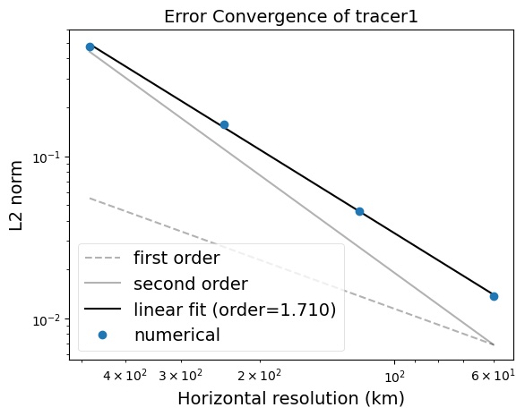
Fig. 10 Tracer higer order convergence example of a cosine bell advected on a sphere showing an order 1.71 convergence rate

Monotonic Flux Limiting Transport for Second Order Horizontal Advection

It is well known that higher order (order 2 and above) scheme for numerically integrating fluxes suffer from dispersive “ripples” in the results particularly near steep gradients. Lower order schemes produce no ripples but suffer from excessive numerical diffusion. Flux-corrected transport (FCT) is a technique which embodies the best of both schemes.

The implementation of a monotonic flux-corrected transport (FCT) in Omega follows a standard algorithm as given in

Zalesak, S. T. (1979). Fully multidimensional flux-corrected transport algorithms for fluids. Journal of Computational Physics, 31(3), 335–362. DOI: 10.1016/0021-9991(79)90051-2

The procedure is as follows given the notation above:

1. Compute \(F^L_{i+1/2}(u\psi)\), the transportive flux by some low order scheme guarenteed to give monotonic (ripple-free) results.

2. Compute \(F^H_{i+1/2}(u\psi)\), the transportative flux by some high order scheme.

3. Define the “antififfusive flux”:

   \[ A_{i+1/2}(u\psi) = F^H_{i+1/2}(u\psi) - F^L_{i+1/2}(u\psi) \]

4. Compute the updated low order (“transported and diffused”) “td” solution:

   \[ w^{td}_i = w^n_i - \frac{1}{\Delta x}[F_{i+1/2}(u\psi) - F_{i-1/2}(u\psi)] \]

5. Limit he \(A_{i+1/2}(u\psi)\) in a manner such that \(w^{n+1}\) as computed below is free of extrema not found in \(w^{td}\) = \(w^n\);

   \[ A^C_{i+1/2}(u\psi) = C_{i+1/2}(u\psi) A_{i+1/2}(u\psi), \quad \quad 0 \leq C_{i+1/2} \leq 1 \]

6. Finally apply hte limited antidiffusive fluxes:

   \[ w^{n+1}_i = w^{td}_i - \frac{1}{\Delta x}[A^C_{i+1/2}(u\psi) - A^C_{i-1/2}(u\psi)] \]

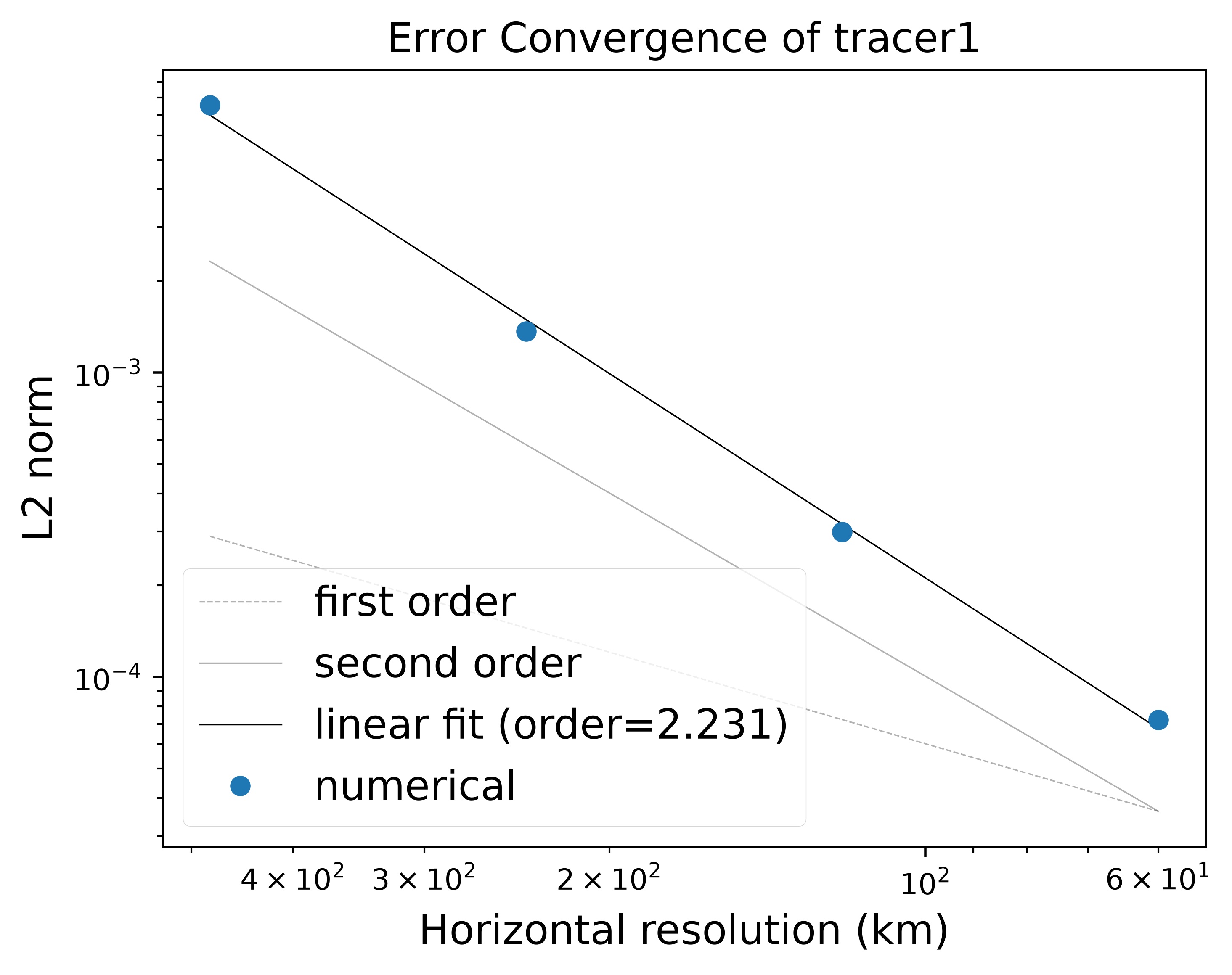
Fig. 11 Tracer higer order convergence example of a cosine bell advected on a sphere with FCT showing an order 2.23 convergence rate

When monotonic flux limiting is used then there are two diagnostic options that can be enabled, HorzTracerFluxLimiterBudgetsEnable and HorzTracerFluxLimiterMonotonicityCheckEnable. The HorzTracerFluxLimiterMonotonicityCheckEnable flag enables a post-transport check that the resulting values are indeed monotone as required by the algorithm and any discrepancies are printed along with information on where they occur.

The HorzTracerFluxLimiterBudgetsEnable option enables the output of two diagnostic fields to the output mesh file. One is the “FCTActiveTracerHorizontalAdvectionEdgeFlux” variable which is the edge flux across every side of every element. The other is the “FCTActiveTracerHorizontalAdvectionTendency” variable which is the cell-centered value of the advection tendency.

Monotonic Flux Limiting Transport Example of Limiting Ripple Effect

The effect of monotonic higher order FCT horizontal transport verses just higher order horizontal transport can be seen in the Polaris test of the slotted cylinder. The cylinder is advected for one revolution under a constant velocity field. The result is advecting the solution back to the original configuration as an exact solution. The difference between the initial condition and the advected solution is the error in the advection scheme. This difference is shown in the following two plots for non-monotonic and monotonic advection.

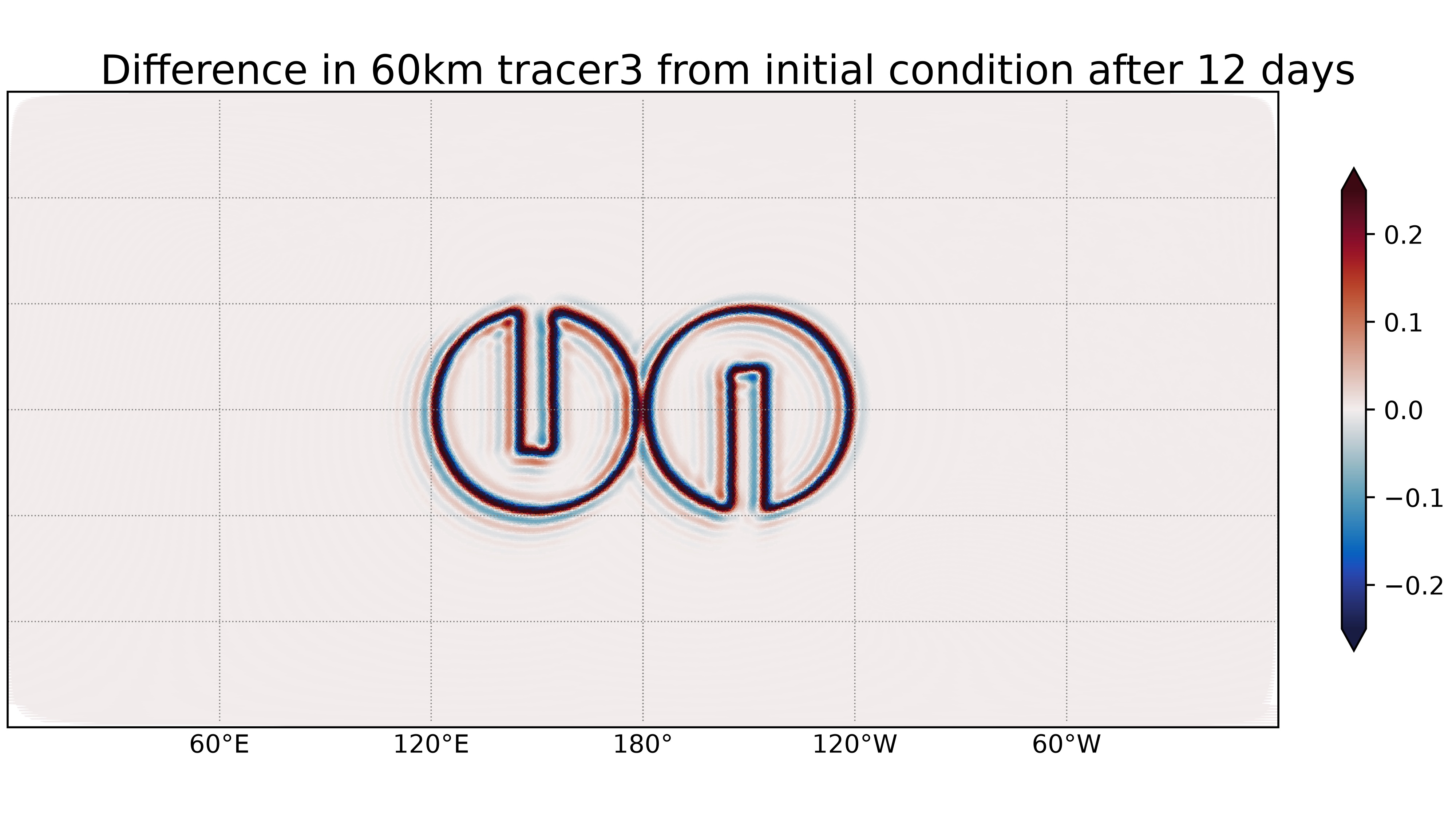
Fig. 12 Error in a tracer higher order convergence example of a slotted cylinder advected on a sphere with the standard third order advection algorithm with no FCT flux correction. Notice the ringing due to the sharp edges of the tracer distribution.

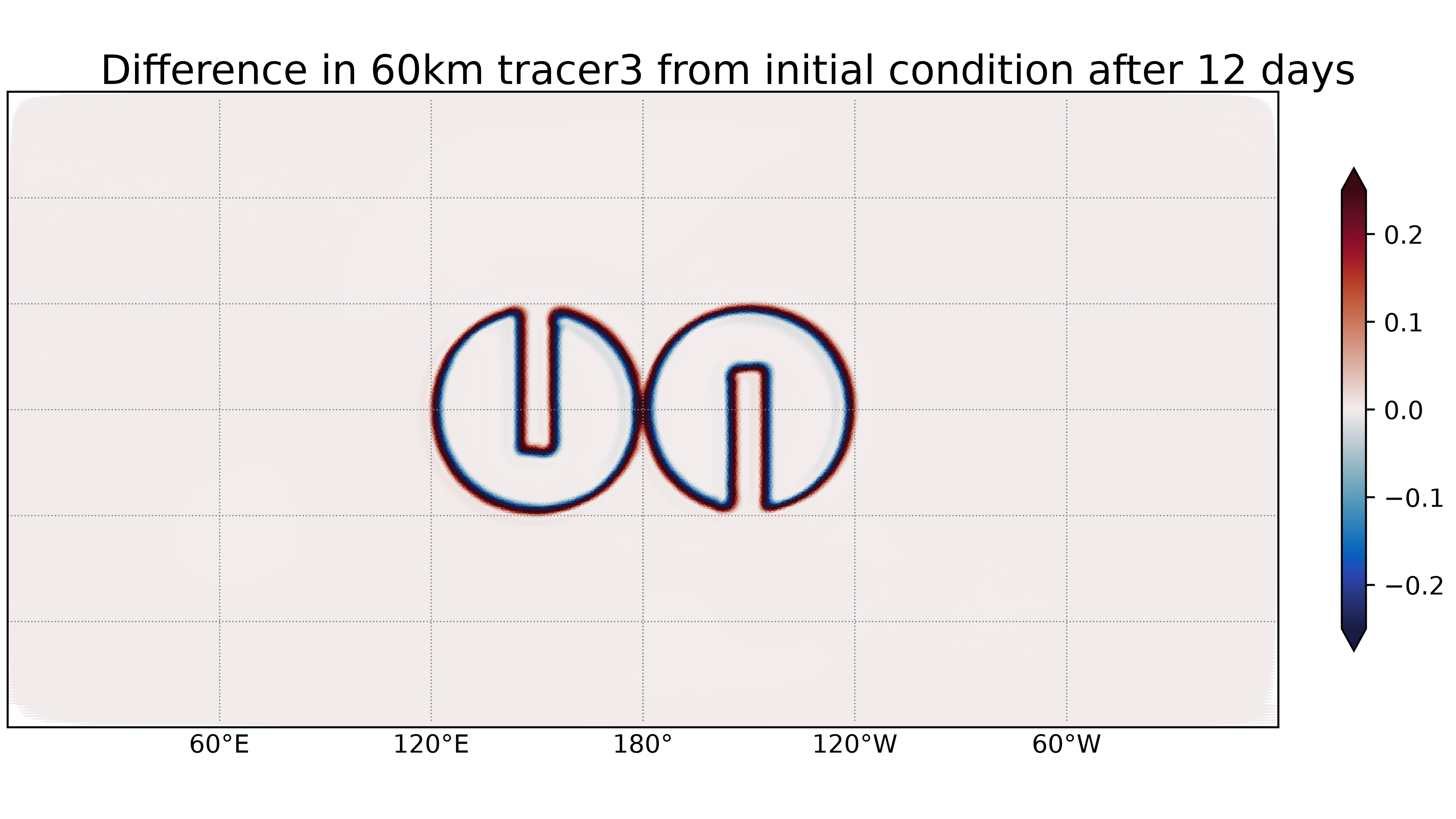
Fig. 13 Error Tracer higher order convergence example of a slotted cylinder advected on a sphere with FCT monotone flux correction. Notice the reduction in ringing around the sharp edges of the tracer distribution.

See Also

Additional information on forcing, including surface stress forcing, surface thickness and tracer flux forcing, and surface tracer restoring, is detailed in Forcing.