The Native3D autoencoder, explained
What n3d/autoencoder.py does, part by part, and what it achieved. MAGGIE Stage 3, 2026-10-16. Code: /pscratch/sd/o/olawale/MAGGIE/E3SM/Native3D/n3d/autoencoder.py (338 lines, 4.07 M parameters).
In short
The autoencoder is a pair of neural networks. The first, the encoder, reads one month of the simulated global ocean and sea ice (104.7 million numbers) and writes a compact code: a table of 29,000 rows, one per 125-km patch of ocean, with 128 numbers in each row. The second, the decoder, answers questions about that month from the code alone: "what was the salinity at this latitude, longitude and depth?" It answers with a value and an error bar, for any point, not only the points the model was stored on.
The code is 28 times smaller than the state and it is what the diffusion prior learns to draw new months from. The decoder is also the bridge to real observations: an Argo float's measurement is a question of exactly the kind it answers.
Why an autoencoder at all
A diffusion model learns by taking a state, adding noise to it, and training a network to remove the noise. It then generates new states by starting from pure noise and removing it step by step, 64 steps in our sampler. If the state were the raw 104.7-million-number field, every one of those steps would be a pass over 104.7 million numbers, and the network would have to learn the structure of the ocean from only 13,824 training months. That is too slow and too data-hungry.
So the prior does not work on the raw state. It works on the code: 3.7 million numbers arranged as a field on a coarse graph. The autoencoder is the translator between the two: it must compress enough to make the prior tractable, and reconstruct well enough that nothing the assimilation cares about is lost. The gate we set for it (Gate G2) was that the reconstruction of held-out months should explain at least 95 % of the variance of every variable.
The same thing as an analogy
Think of the ocean as a country of 465,044 towns (the mesh cells). Each town keeps a logbook with 335 entries: the temperature, salt and currents at each of its 64 floors from the surface down to the seabed, plus the sea level and the ice at the top, plus where the town is and how deep its seabed goes.
- Every town writes a 128-word summary of its logbook (step 2). The same small writer is used for every town, so the summaries are comparable.
- Every town reads its six neighbours' summaries and revises its own, twice (step 3). Now each summary also says what is going on within 90 km.
- The country is divided into 29,000 districts of about 16 towns, drawn so that no district crosses land (step 4). Each district merges its towns' summaries into one 256-word district report.
- Districts hold four rounds of regional meetings (step 5). In each round, a district reads the reports of its 32 nearest districts, paying more attention to some than to others, and revises its own. After four rounds a district report reflects the state of the ocean about 1,000 km around it.
- The reports are condensed to 128 words each. The 29,000 condensed reports are the code (step 6).
- To answer a question ("salt at this spot, 850 m down"), a clerk writes the question in a fixed form, then reads the report of the district the spot is in and the nine districts touching it, twice, weighing each by its position relative to the spot (steps 7 and 8). The clerk answers with a number and a confidence (step 9).
The whole machine is trained by asking 390,000 random questions about each month and comparing the clerk's answers with the real logbooks. Every part, writer, meetings and clerk, is adjusted together so the answers get better; nobody tells the district reports what to contain. That is what "learned" means here: the 128 words per district are whatever turned out to be most useful for answering questions.
The picture
docs/make_ae_simple.py.In the code's own words: the encoder (steps 1–6) reads a whole state at once (no batch dimension; one state per GPU) and produces z of shape (29,000, 128); the decoder (steps 7–9) takes z and a set of queries and returns two numbers per query. The sections below follow the same nine steps, each with a plain statement of what happens, then the actual layer names and sizes.
Follow one point through the machine
Take a real place: 38° N, 60° W, in the Gulf Stream south of Nova Scotia, and ask for the salinity 850 m down in May 1980. Here is what happens to that one number.
| step | what happens to our point | size at this step |
|---|---|---|
| 1 | The point sits in mesh cell number 212,345 (say), at level 40 of that cell's column (level 40 spans 800–900 m). The stored value is a z-score: how unusual the salinity is for a May at that depth there, in units of the typical May variation at that depth. Suppose it is +1.3. | one of 104.7 M numbers |
| 2 | The cell's whole column (64 levels × T, S, U, V, with zeros below the 4,100 m seabed and a mask saying which levels are water), its sea level, its ice (none here), and its static facts (position, seabed depth, 23 hops from the coast, cell area) make 335 numbers. The column MLP turns them into a 128-number token. Our +1.3 is now spread across those 128 numbers together with everything else in the column. | 465,044 × 128 |
| 3 | The cell's six neighbours send their tokens, each shifted by a small learned function of where they lie (one is 30 km east, one 30 km north-east, …). The cell averages the messages and updates its token. Twice. The token now knows there is a sharp front 60 km to the north. | 465,044 × 128 |
| 4 | The cell belongs to latent node 8,811, whose patch is 17 cells reachable through water. The node's token is an MLP of three things: the token of the node's own central cell, the mean of the 17 tokens and the element-wise maximum of the 17 tokens. | 29,000 × 256 |
| 5 | Node 8,811 attends to itself and its 31 nearest nodes (the 6 touching it and the ring beyond, out to ≈ 250 km). Four times, each time with a different learned way of weighing them and a position-aware bias. The Gulf Stream's whole meander, 1,000 km of it, is now reflected in the node. | 29,000 × 256 |
| 6 | A final linear layer condenses the node to 128 numbers. This row of z is where "salinity +1.3 at 850 m at 38° N 60° W" now lives, mixed with the temperature, the currents, the sea level and the other 1,087 wet points of the patch. | 29,000 × 128 |
| 7 | To get it back we write the question: the unit vector of 38° N 60° W as 36 sine/cosine numbers, the depth 850 m (on a log scale) as 12 more, the 8 static facts of the cell, and a learned 32-number tag for "salinity". An MLP turns these 88 numbers into a 128-number question token. | 88 → 128 |
| 8 | The question token attends to the 10 latent rows around it: node 8,811 and its 6 to 9 touching nodes, each read through a linear layer together with the node's static facts, and each weighted by how it lies relative to the point (the node 90 km downstream matters differently from the one upstream). Two such blocks. | reads 10 × 128 |
| 9 | The head returns two numbers: the value, say +1.21, and a log-variance, say −2.4, meaning σ = 0.30. The reconstruction is 0.09 below the truth and the model's own error bar says ±0.30, which is honest: at 850 m in the Gulf Stream, 125-km patches cannot pin a front to better than that. | 2 |
For the full-state evaluation this is repeated for every one of the 25.1 million wet points and 11 variables, in chunks of 500,000 questions; it takes about a minute per month on one GPU.
1. Inputs: what a cell knows (cell_inputs)
What happens. Every column of water is written out as one fixed-length list of 335 numbers, so that one and the same small network can read every column.
| part | numbers | what |
|---|---|---|
| water column | 256 | T, S, U, V at the 64 levels, as stored z-scores (anomaly from the monthly climatology divided by the per-level standard deviation); dry levels are 0 |
| wet mask | 64 | 1 where the level is water, so the network can tell a zero from a dry level |
| sea-surface height | 1 | z-score |
| sea ice | 4 | concentration, volume, snow volume, surface temperature, divided by ICE_SCALE = (1, 1, 0.1, 10) to be of order one |
| ice velocity | 2 | the vertex velocities averaged over the cell's 5–6 vertices (_ice_v_cell), divided by 0.1 m/s |
| static features | 8 | from tokens.build_static: unit vector (3), log bottom depth, wet fraction, ice-shelf flag, hops from the coast, log cell area |
The column is written into a dense (cells × 64 × 4) array through the index of wet points (wet_flat), which is how the cell-major wet-only storage of the data meets the per-cell view of the network. Stored z-scores are already of order one, which is why there is no normalisation layer here. "Z-score" throughout means: the value minus the climatological mean for that month and place, divided by the standard deviation at that depth, so a +2 at 4,000 m (where the variation is a few thousandths of a degree) is as unusual as a +2 at the surface (where it is a degree or more).
2. Column MLP: one token per cell (cell_in)
What happens. A two-layer network reads the 335 numbers of a column and writes a 128-number summary, the cell's token. It sees the whole column at once, so it can describe a thermocline or a cold deep layer as a shape rather than level by level.
h = MLP(335 → 256 → 128)(inputs) # (465,044, 128)A variant with 1-D convolutions over depth before this MLP (model_ae.column: conv, runs ae128c and ae128v) was tested and rejected: it learned more slowly in every depth band and cost 28 % more time. The option remains in the code with mlp as the default.
3. Message rounds: cells talk to their neighbours (msg, rel_msg, upd)
What happens. Each cell collects a message from each of its 5 or 6 neighbours, averages them, and revises its token. Doing this twice lets every cell know what the ocean looks like two cells away, about 90 km, before the detail is pooled away in the next step.
for round in 1, 2:
    nb  = W·h[neighbours] + R·rel          # (465,044, 6, 128): the 5–6 cells on cell
    agg = GELU(mean over valid neighbours of nb)
    h   = h + MLP([h | agg])               # (465,044, 2·128 → 128 → 128)
Two rounds of message passing on cells_on_cell (the mesh adjacency, 2.8 million directed edges). Each neighbour's token is passed through a linear map W and offset by a linear function of the neighbour's displacement in the cell's local east–north frame, in units of one cell spacing (REL_CELL = 0.005 rad ≈ 30 km), so the cell knows which message came from the east and which from the north. The messages are deliberately linear per edge: a hidden activation on each of the 2.8 M edges × 128 channels would not fit next to the rest of the state on a 40 GB GPU. The nonlinearity sits after the mean.
4. Pooling: regions become latent nodes (pool, members)
What happens. The 465,044 cell tokens are merged into 29,000 node tokens, one per patch of about 16 cells. This is where most of the compression happens: 16 cells become one row.
g = MLP([h[latent cell] | mean of members | max of members]) # (29,000, 3·128 → 256 → 256)The latent graph (n3d/graph.py) picks 29,000 latent cells by farthest-point sampling (median spacing 124 km) and assigns every ocean cell to the nearest latent cell by a breadth-first search through water, so a region never crosses land: a cell on the Pacific side of Panama belongs to a Pacific node even if an Atlantic node is nearer as the crow flies. Regions hold 2 to 33 cells (median 16). They are stored as a padded (29,000 × 33) table; the pooling is a gather, a masked mean and a masked max over that table. The mean carries the typical state of the patch, the max carries its extremes (a front or an eddy that the mean would blur), and the latent cell's own token is kept as a third input so the node knows its centre as well as its region.
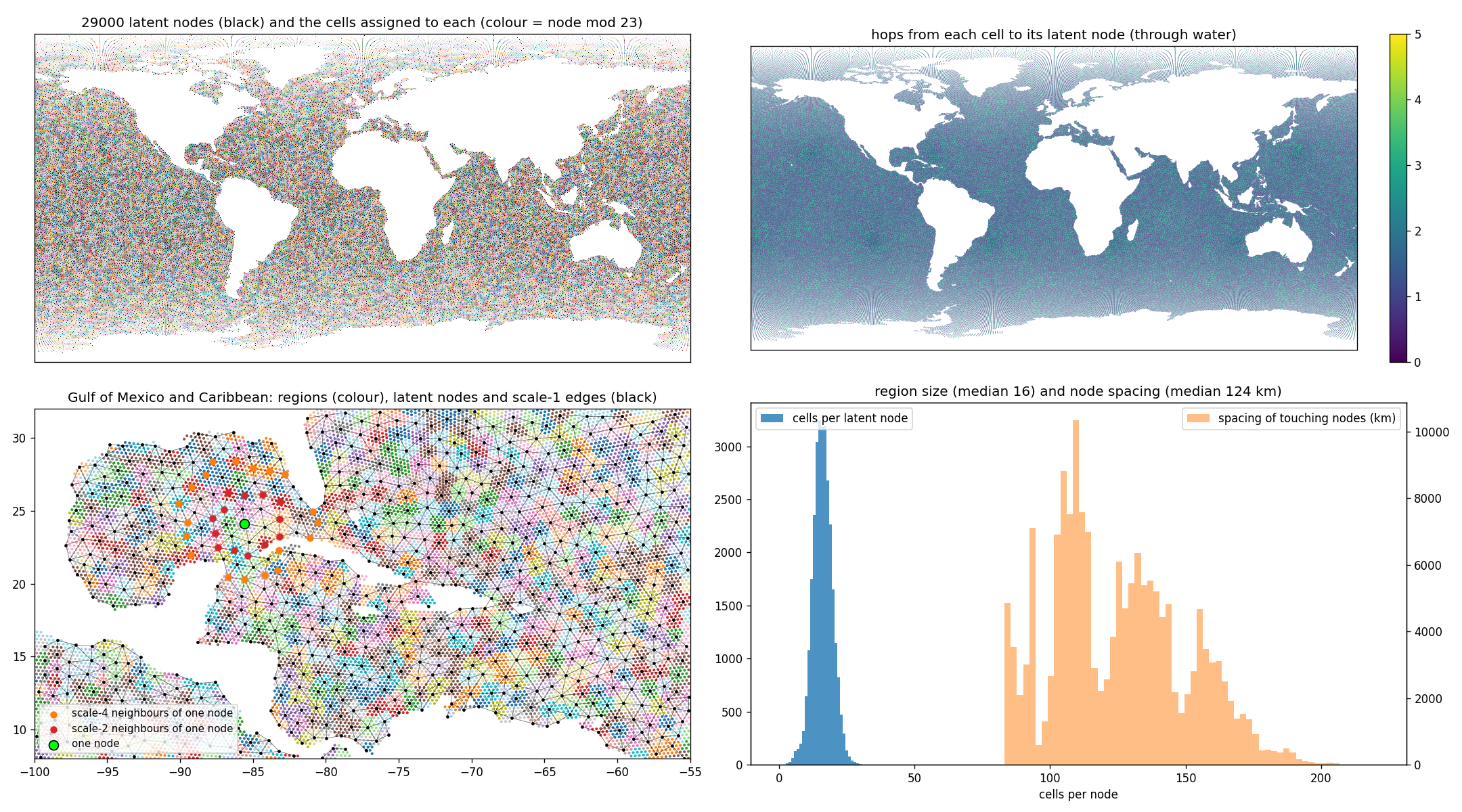
figures/graph/latent_graph.png).5. Latent attention: nodes see their rings (enc_blocks, NeighbourAttention)
What happens. Each node looks at its 32 nearest nodes and decides, separately for each of four "heads", how much to take from each of them; then revises its token. Four such blocks. After them a node reflects the ocean about 1,000 km around it, so basin-scale structure (a gyre, a meander, a warm pool) is in the code and not only local detail.
for block in 1..4:
    g = g + Attn(LN(g) → its 32 table tokens, bias = MLP(rel) per head)
    g = g + MLP(LN(g))                      # 256 → 1024 → 256
z = Linear(LN(g))                            # (29,000, 128)
"Attention" here means: the node computes a weight for each of its 32 candidates from the match between its own token and theirs, adds a bias that depends on where the candidate lies relative to the node (REL_LAT = 0.02 rad ≈ 125 km), turns the weights into fractions that sum to one, and takes that weighted mix of the candidates' tokens. The table of 32 is fixed per node: itself, its scale-1 neighbours, then scale-2 neighbours, padded with −1 where the ring is short. The NeighbourAttention class does this with one einsum over (node, key, head, channel); there is never a 29,000 × 29,000 matrix. The final LayerNorm and linear map produce the 128 latent channels.
In training a small Gaussian noise (z_noise 0.1) is added to z and a tiny L2 penalty (z_l2 10-3) keeps its scale of order one; both exist for the prior's sake, so that the latent space is smooth (a slightly wrong code still decodes to a sensible ocean) and not arbitrarily scaled. The trained latents have a channel standard deviation of 2 to 3.
6. Query decoder: any point, any depth, any variable (decode)
What happens. A question (where, how deep, which variable) is turned into a token, that token reads the 10 code rows around the place, and a small head writes the answer: a value and how sure it is.
q   = MLP([Fourier(xyz) 36 | Fourier(log depth) 12 | static of the cell 8 | variable embedding 32])   # 88 → 128
tok = Linear([z | static of the latent cell])                                                          # 136 → 128
for block in 1, 2:
    q = q + Attn(LN(q) → the 10 latent tokens of the query's owner node, bias = MLP(rel))
    q = q + MLP(LN(q))
value, log-variance = Head(q)                                                                          # 128 → 128 → 2
A query is a tuple (unit vector on the sphere, depth in metres, cell, variable id). Its position enters as sine and cosine features at 6 frequencies each for x, y, z and for the log-scaled depth (tokens.query_features, 56 geometry numbers). Sines and cosines are used because a network finds it much easier to tell two nearby positions apart from a set of waves of different wavelengths than from three raw coordinates. The question also carries the static features of the cell it falls in and a learned 32-dimensional tag for which of the 11 variables is wanted. It then attends, in two cross-attention blocks, to the 10 latent tokens around it: the owner node of its cell and that node's scale-1 neighbours (k_dec 10, table_dec), with the same displacement bias as the encoder. The head returns a value and a log-variance. Ice variables are decoded at depth 0; ice velocity at vertex positions, with any adjacent cell as the query's cell.
Because the decoder is a function and not a grid, the same weights serve three jobs: reconstructing the full state (25 million queries, in chunks of 500,000), evaluating the model at observation positions during guidance, and comparing samples of the prior with data. The decoder's capacity is small on purpose (0.46 M of the 4.07 M parameters): most of the work is in the latent, and a small decoder keeps the full-state decode at about 7 s per variable.
7. Training queries: what is decoded each step (sample_queries)
What happens. Decoding all 104.7 million targets at every training step would be far too slow, so each step asks a random sample of 390,000 questions per state and checks the answers against the stored values.
| kind | queries | drawn from |
|---|---|---|
| ocean | 300,000 | wet points × a random variable among T, S, U, V. With level_balance 0.5 half of them pick a level uniformly first, then a wet point of that level, so the deep levels (few cells, tiny variance) get as many examples as the surface (runs ae128b, ae128g) |
| vgrad | 100,000 pairs | a wet point with a wet point directly below it, in the same column, same variable; the loss uses their difference (run ae128g) |
| ssh | 30,000 | cells, depth 0 |
| ice | 30,000 | cells poleward of 40°, one of the four ice fields |
| ice_v | 30,000 | vertices poleward of 40°, u or v |
The targets come straight from the stored state, so no interpolation is involved: the query depth is the mid-depth of the level the point sits in. Uniform sampling over wet points favours the upper ocean (the top 200 m hold about a third of all wet points and most of the variance); level balancing was the fix for the abyss: without it, the model saw a 5,000 m point once for every twenty surface points and learned the abyss poorly.
8. Loss: Gaussian likelihood plus a vertical-gradient term (loss)
What happens. The model is scored on each answer by how far the value is from the truth relative to its own error bar, plus a penalty for claiming a large error bar. This rewards answers that are close and error bars that are neither boastful nor timid. A second term scores the difference between vertically adjacent answers, which is what makes the model get the layering of the ocean right.
nll   = ½ · ((y − μ)² · exp(−logvar) + logvar)          mean over all queries, logvar clamped to [−7, 5]
vgrad = mean over pairs of ((μ_below − μ) − (y_below − y))²
loss  = nll + vgrad_weight · vgrad + z_l2 · mean(z²)
The first line is the negative log-likelihood of a Gaussian with the predicted mean and variance. It makes the decoder honest about its uncertainty: the variance cannot shrink without the error shrinking too, and the 1σ coverage in evaluation is 0.74–0.78 (0.68 would be perfect; the model is slightly wide). The vertical-gradient term (ae128g, weight 5) decodes the two points of each vertical pair and penalises the error of their difference. Since the mean-square of the stored vertical difference is only 0.11, a model that got each point right to 0.3 could still have the stratification wrong; this term asks for the right stratification directly. It is what removed the near-surface dip of the R² profile (the top 50 m, where the mixed layer sits on the thermocline).
forward = loss at the end of the file is what lets DistributedDataParallel wrap the module: each GPU calls forward on its own state and the gradients are averaged across the four GPUs of a node.
Why these numbers
Why 29,000 nodes
About 125 km spacing: enough to hold the gyres, boundary currents and the ice edge, and 16× fewer rows than the mesh. More nodes would make the prior proportionally slower (the prior's cost scales with the number of nodes); fewer would blur the western boundary currents entirely. The number is set in config.yaml (graph.n_latent) and everything else adapts to it.
Why 128 numbers per node
Each row stands for about 3,600 stored numbers. 128 is enough that T, S, U, V over 64 levels can be told apart by the decoder (R² 0.95–0.98) while keeping the code at 3.7 M numbers, small enough that the prior's attention over 29,000 tokens fits in memory. A 256-channel latent is the first thing to try if the abyss needs more room.
Why a question-answering decoder
Real observations are not on the mesh: an Argo profile reports at its own depths, a satellite at its own footprint. A decoder that answers at any (position, depth, variable) can be compared with them directly, with no interpolation step whose errors would have to be modelled separately. It also makes the decoder's size independent of the output resolution.
Why 10 tokens per question
The owner node and its touching ring cover about 250 km around the point. The encoder has already put the larger-scale context into those tokens (step 5), so the decoder need not look further. Reading only 10 rows keeps a full-state decode (25 million questions) to about a minute.
Why an error bar
The guidance will pull the prior towards observations through this decoder. It needs to know how far to trust a decoded value against a measured one: a decoded salinity in the Gulf Stream deserves less weight than one in the quiet subtropical interior. The predicted variance is that weight, and the Gaussian loss is what makes it calibrated.
Why z-scores per level
The abyss varies by thousandths of a degree, the surface by degrees. Without per-level standardisation the loss would be dominated by the surface and the deep ocean would be invisible to the model. With it, every level counts by its own variability, which is also why R² is reported in stored units.
Parameters and cost
| part | parameters | note |
|---|---|---|
column MLP (cell_in) | 0.12 M | 335 → 256 → 128 |
| 2 message rounds | 0.13 M | linear messages, update MLPs |
| pooling | 0.16 M | 384 → 256 → 256 |
| 4 latent attention blocks | 3.16 M | d 256, 4 heads, K 32; most of the model |
| latent head | 0.03 M | 256 → 128 |
| query decoder (2 blocks, heads, embeddings) | 0.46 M | d 128, k_dec 10 |
| total | 4.07 M |
One training step on one state takes 0.32 s on an A100 (forward 0.1 s, backward 0.2 s) and about 20–25 GB. Four states per step on four GPUs give 10–11.5 states/s; 100,000 steps are 10 hours, three or four interactive allocations. The first version of the model took 4.2 s per state: 94 % of it was the sort-based backward of fancy indexing (x[idx]) over 2.8 M cell edges and 3.9 M decoder keys. Replacing those gathers by F.embedding (gather at the top of the file), whose backward is a segment reduction, and replacing scatter pooling by the padded member table, brought it to 0.32 s.
Results: three runs, one winner
All runs: 100,000 steps, 4 states per step, learning rate 2·10-4 with 1,000 warm-up steps, EMA weights evaluated. Full-state R² is computed by decoding every wet point of 8 held-out states (val = years 1990–94 starts, test = 1996–99), in stored units, so every level counts by its own variance.
How to read R². It is the fraction of the variance of the true field that the reconstruction explains: 1.0 would be a perfect copy, 0 would be no better than predicting the climatological mean everywhere. 0.978 for temperature means the reconstruction's errors have 2.2 % of the variance of the real anomalies, or an RMS error of about 15 % of the RMS anomaly. The gate, 0.95, corresponds to an RMS error of 22 %.
| run | what changed | T | S | U | V | SSH | ice conc. | T 0–200 m | T > 2 km |
|---|---|---|---|---|---|---|---|---|---|
| ae128 | baseline | 0.970 | 0.968 | 0.946 | 0.930 | 0.996 | 0.998 | 0.974 | 0.906 |
| ae128b | + level balance 0.5 | 0.972 | 0.970 | 0.947 | 0.932 | 0.996 | 0.998 | 0.970 | 0.933 |
| ae128g | + level balance + vertical gradient | 0.978 | 0.977 | 0.950 | 0.936 | 0.995 | 0.997 | 0.984 | 0.936 |
| ae128g on the test years | 0.975 | 0.964 | 0.951 | 0.937 | 0.996 | 0.996 | 0.980 | 0.901 | |
Gate G2 (held-out R² ≥ 0.95) is met by T, S, U, SSH and all ice fields on both held-out periods. V is at 0.936, held back only by the abyss (0.85 below 2 km). Test values sit close to validation values, so nothing is memorised from the training years. Precision is not the limit: decoding ae128g in fp32 instead of bf16 changes no R² by more than 0.0003.


Engineering notes worth knowing
Geometry lives in buffers, not checkpoints
Every table (adjacency, displacements, member regions, latent tables, wet indices) is a non-persistent buffer rebuilt from mesh.npz and graph_29000.npz at construction. Checkpoints hold only the 4 M parameters; load_weights drops the buffers that older checkpoints carried.
Padding instead of ragged tensors
Pentagon cells have 5 neighbours, latent rings vary in size, regions hold 2–33 cells. Everything is padded with −1 and masked: neighbours in the mean, keys in the softmax (−∞), members in mean and max. gather clamps the −1 to 0 and the mask removes it afterwards.
Local frames everywhere
Displacements are expressed in each point's own east–north frame (local_basis, with a fixed basis at the poles), scaled to one cell spacing for the mesh and one latent spacing for the coarse graph. The same relative-position bias serves the encoder's rings and the decoder's cross-attention.
One state per GPU, no batch dimension
The encoder's tensors are (cells, …) and (latent nodes, …); a batch would be a loop. DDP averages gradients across GPUs; batch in the config is the number of GPUs.
bf16 autocast
Training and evaluation run under bf16 autocast with fp32 weights, optimiser and loss. An fp32 evaluation of the final model reproduced every R² to three decimals.
What the decoder cannot do
It has no access to the input state, only to z. Anything finer than the 124 km latent spacing (eddies, the Gulf Stream's edge, river plumes) is reconstructed as the smooth field the latent can hold, which is where the remaining error sits.
Glossary
| word | meaning here |
|---|---|
| state | one month of the simulated ocean and sea ice on the native mesh: 104.7 million numbers |
| cell, column | one hexagon of the mesh (about 30 km across) and the water beneath it, up to 64 levels deep |
| wet point | one (cell, level) pair that is water; 25.1 million of them |
| z-score, stored units | a value minus its monthly climatological mean, divided by the standard deviation at that depth; what the data files hold |
| token | a fixed-length list of numbers that describes one thing (a cell, a node, a question); 128 or 256 numbers here |
| latent, code, z | the 29,000 × 128 table the encoder writes and the decoder reads; "latent" because its meaning is learned, not assigned |
| node, patch, region | one row of the code and the ≈ 16 cells it stands for |
| MLP | a small fully connected neural network: a few layers of "multiply by a matrix, add, apply a bend" |
| attention | a layer in which a token takes a weighted mix of other tokens, choosing the weights from how well they match it and where they lie |
| query, question | a request to the decoder: a position, a depth and a variable name |
| log-variance, error bar | the decoder's second output: the logarithm of the variance it assigns to its own answer; σ = exp(½ log-variance) |
| R² | fraction of the variance of the truth explained by the reconstruction; 1 = perfect |
| Gate G2 | the project's acceptance test for the autoencoder: held-out R² ≥ 0.95 per variable |
| EMA weights | a slowly moving average of the trained weights, used for evaluation and for the prior; smoother than the last step's weights |
Source files: n3d/autoencoder.py, n3d/tokens.py, n3d/graph.py, train_ae.py, evaluate_ae.py; results in PLAN.md §6 and the walkthrough. Schematic drawn by docs/make_ae_simple.py.