Inside SamudrACE C1A0
Circuits, law witnesses and error agreement for the E3SMv3 coupled emulator (SFNO atmosphere + Samudra ocean), finished at scale on Perlmutter against E3SM truth, scored only on years the model never saw (1995–1999, 2040–2049). Rules were preregistered before results (PREREG.md). This page is rebuilt from the result JSONs. Participants: start with HACKATHON.md and the repo.
Headline so far
samudra Patchable adapter, EdgePatch semantics) gives skip.0 share 0.854 on 7 states of 2045 (localize.py: 0.86)Setup, data and checks
Model and lineage
| Checkpoint | HF mahf708/e3smv3-lr-hist-samudrace@rc1 checkpoints/C1A0.tar, md5 a5082a9aec1243e37e0820a99e77d059 |
| Training run | E35-CFT S01: 25 epochs coupled fine-tune (4 coupled steps, ensemble CRPS), EMA weights |
| Atmosphere | NoiseConditioned SFNO, 8 blocks × 384, big skip, isotropic noise (32 ch); init E02-FT S01. 6 h step. Corrector: dry air, moisture budget, positivity |
| Ocean | Samudra U-Net 280/380/480/520, InstanceNorm; init E11-FT S01 (= the hackathon E11 archive ocean). 5-day step; FLUS is an input; corrector never touches sst |
| Coupling | ocean fluxes = atmosphere outputs averaged over 20 inner steps; the atmosphere sees the ocean's current SST |
| Other release checkpoints | C0A0 = E30-CFT S03 (no CO₂; ocean E11-FT S03); C1A1 = E31-CFT S01 (CO₂ + aerosol; atmosphere E05-FT S01, ocean E11-FT S01, same as C1A0) |
Truth data and splits
| Run | v3.LR.historical_0101.aigo: EAM 6-hourly, MPAS-O/SI 5-day means, 1940–2065, 1° Gaussian (C1A0's grid) |
| Train | 1940-01-06 … 1990-01-01 and 2000-01-06 … 2040-01-01 |
| Validation | 1990–1994 (also used to pick the checkpoint) |
| Held out (scored here) | 1995–1999 and 2040–2049; fit years 1995–97 / 2040–44, score years 1998–99 / 2045–49 |
| Laptop states | 1985, 2015 = training years; used only to reproduce laptop numbers |
Exactness and reproducibility checks
| check | result |
|---|---|
| common.Graph vs Samudra.forward (A100) | max |diff| 0.0 (bitwise) |
| SamudraReplay vs Samudra.forward | max |diff| 0.0 (bitwise) |
| same-seed fme coupled steps (all tensors, all outputs) | bitwise identical |
| de-leak switch at load time (CombinedFluxConfig FLUS := 5.67e-8·sst⁴) | works without editing the checkpoint; ocean FLUS / emission median 0.9997; control − de-leak FLUS 5.6 W/m² RMS (step 0), 7.3 (step 1) |
| TF32 (CUDA default) vs fp32 | TF32: batch-of-4 vs single 0.021 K max; fp32: 4.3e-05 K; fp32 vs deployed TF32 output 0.06 K max |
| truth-forced ocean input builder vs fme packing of the 1995-01-01 truth IC | all state channels identical; only the 9 flux channels differ (truth vs coupled-atmosphere fluxes), as expected |
Reproduce
bash setup_env.sh
python -m hc.capture data/smoke/A --steps 2 --atm-pred
python -m hc.capture data/smoke/B --steps 2 --atm-pred
python -m hc.capture data/smoke/D --steps 2 --deleak
python phase0/smoke.py data/smoke/A data/smoke/B data/smoke/D
python phase0/numerics_check.py data/smoke/A
Results: smoke.json numerics_check.json flus_slope.json
Idea 1 · The ocean reads FLUS as an SST thermometer
Question. Raising upward longwave (FLUS) at the ocean's input warms its next SST (wrong sign on 99.8% of open ocean). Is this a target leak, i.e. is the training-time FLUS (a 5-day mean over the window being predicted, the coupler's emission from that window's SST) a legitimate predictor of the target? If so, does the model's response match the truth relation, and can it be removed without breaking the lawful fluxes?
F1 (a) · Alignment of FLUS with εσT⁴ in truth
FLUS[w] is the 5-day mean the ocean receives with window w (MPAS = what training fed; EAM = the atmosphere's own). ε fitted on fit years over open ocean, scored on score years. Five SST definitions: previous-window mean (what the ocean reads), target-window mean, window-mean TS⁴ (6-hourly EAM), instantaneous TS at window start and end.
| block | FLUS source | SST definition | ε | RMS (W/m²) | pooled R² | per-cell R² (median) |
|---|---|---|---|---|---|---|
| 1990s | FLUS | prev_window_mean_sst[w-1] | 0.9883 | 22.28 | 0.8449 | 0.744 |
| 1990s | FLUS | target_window_mean_sst[w] | 0.9884 | 22.21 | 0.8459 | 0.770 |
| 1990s | FLUS | window_mean_TS^4 | 0.9948 | 16.50 | 0.9149 | 0.944 |
| 1990s | FLUS | window_start_TS | 0.9956 | 16.77 | 0.9122 | 0.950 |
| 1990s | FLUS | window_end_TS | 0.9957 | 16.86 | 0.9113 | 0.951 |
| 1990s | FLUS_eam | prev_window_mean_sst[w-1] | 0.9957 | 9.17 | 0.9673 | 0.937 |
| 1990s | FLUS_eam | target_window_mean_sst[w] | 0.9958 | 8.83 | 0.9697 | 0.961 |
| 1990s | FLUS_eam | window_mean_TS^4 | 1.0003 | 1.12 | 0.9995 | 1.000 |
| 1990s | FLUS_eam | window_start_TS | 1.0010 | 4.50 | 0.9921 | 0.988 |
| 1990s | FLUS_eam | window_end_TS | 1.0011 | 4.48 | 0.9922 | 0.988 |
| 2040s | FLUS | prev_window_mean_sst[w-1] | 0.9887 | 22.37 | 0.8516 | 0.781 |
| 2040s | FLUS | target_window_mean_sst[w] | 0.9887 | 22.29 | 0.8527 | 0.806 |
| 2040s | FLUS | window_mean_TS^4 | 0.9946 | 17.03 | 0.9140 | 0.946 |
| 2040s | FLUS | window_start_TS | 0.9954 | 17.27 | 0.9115 | 0.952 |
| 2040s | FLUS | window_end_TS | 0.9955 | 17.36 | 0.9106 | 0.954 |
| 2040s | FLUS_eam | prev_window_mean_sst[w-1] | 0.9961 | 8.91 | 0.9708 | 0.948 |
| 2040s | FLUS_eam | target_window_mean_sst[w] | 0.9962 | 8.53 | 0.9732 | 0.970 |
| 2040s | FLUS_eam | window_mean_TS^4 | 1.0003 | 1.15 | 0.9995 | 1.000 |
| 2040s | FLUS_eam | window_start_TS | 1.0010 | 4.63 | 0.9921 | 0.989 |
| 2040s | FLUS_eam | window_end_TS | 1.0011 | 4.59 | 0.9923 | 0.989 |
| 1980s_train_contrast | FLUS | prev_window_mean_sst[w-1] | 0.9883 | 22.29 | 0.8442 | 0.746 |
| 1980s_train_contrast | FLUS | target_window_mean_sst[w] | 0.9883 | 22.22 | 0.8452 | 0.771 |
| 1980s_train_contrast | FLUS | window_mean_TS^4 | 0.9949 | 16.63 | 0.9132 | 0.946 |
| 1980s_train_contrast | FLUS | window_start_TS | 0.9957 | 16.88 | 0.9107 | 0.953 |
| 1980s_train_contrast | FLUS | window_end_TS | 0.9958 | 16.96 | 0.9097 | 0.954 |
| 1980s_train_contrast | FLUS_eam | prev_window_mean_sst[w-1] | 0.9957 | 9.00 | 0.9682 | 0.937 |
| 1980s_train_contrast | FLUS_eam | target_window_mean_sst[w] | 0.9957 | 8.66 | 0.9706 | 0.961 |
| 1980s_train_contrast | FLUS_eam | window_mean_TS^4 | 1.0003 | 1.12 | 0.9995 | 1.000 |
| 1980s_train_contrast | FLUS_eam | window_start_TS | 1.0010 | 4.52 | 0.9920 | 0.989 |
| 1980s_train_contrast | FLUS_eam | window_end_TS | 1.0011 | 4.49 | 0.9921 | 0.988 |
Reading: EAM's FLUS is exactly εσ⟨TS⁴⟩ over its window (RMS 1.1 W/m²). MPAS FLUS carries a spatially varying offset against every SST definition (pooled RMS 16–22 W/m²) that hides the time relation; per-cell R² favours the target window (0.770 vs 0.744 in the 1990s). The preregistered supporting criterion (end beats start by > 20% pooled RMS) is not met.
F1 (b) · The conditional slope in truth
Per open-ocean cell (ice-free in every window): ΔSST = sst[w] − sst[w−1] regressed on the five window-w fluxes, sst[w−1], annual + semiannual harmonics and an intercept (OLS, Newey–West lag 6). K per 100 W/m² of warming flux (FLUS, LHFLX, SHFLX enter with −1), so the thermometer sign is negative. The Frisch–Waugh restatement agrees to 5e-9 (one number, not two).
| block | years | flux | area mean | median | 5–95% | area frac. negative | area frac. |z|>2 |
|---|---|---|---|---|---|---|---|
| 1990s | score | FLUS | -17.17 | -16.952 | [-20.36, -15.87] | 0.995 | 0.995 |
| 1990s | score | FLDS | +0.02 | +0.003 | [-0.03, +0.05] | 0.382 | 0.177 |
| 1990s | score | FSNS | -0.00 | +0.002 | [-0.01, +0.02] | 0.290 | 0.232 |
| 1990s | score | LHFLX | -0.12 | +0.002 | [-0.01, +0.02] | 0.337 | 0.280 |
| 1990s | score | SHFLX | +0.08 | -0.000 | [-0.05, +0.05] | 0.498 | 0.215 |
| 1990s | fit | FLUS | -17.24 | -16.931 | [-20.36, -15.91] | 0.995 | 0.995 |
| 1990s | fit | FLDS | +0.00 | +0.003 | [-0.03, +0.03] | 0.400 | 0.152 |
| 1990s | fit | FSNS | -0.06 | +0.002 | [-0.01, +0.01] | 0.326 | 0.196 |
| 1990s | fit | LHFLX | -0.10 | +0.002 | [-0.01, +0.02] | 0.333 | 0.273 |
| 1990s | fit | SHFLX | +0.14 | -0.000 | [-0.04, +0.06] | 0.507 | 0.190 |
| 2040s | score | FLUS | -17.01 | -16.770 | [-20.18, -15.72] | 0.995 | 0.995 |
| 2040s | score | FLDS | -0.02 | +0.002 | [-0.03, +0.04] | 0.426 | 0.171 |
| 2040s | score | FSNS | +0.00 | +0.001 | [-0.01, +0.01] | 0.343 | 0.200 |
| 2040s | score | LHFLX | -0.18 | +0.002 | [-0.01, +0.02] | 0.299 | 0.358 |
| 2040s | score | SHFLX | +0.12 | -0.000 | [-0.06, +0.06] | 0.512 | 0.246 |
| 2040s | fit | FLUS | -17.13 | -16.816 | [-20.23, -15.72] | 0.995 | 0.995 |
| 2040s | fit | FLDS | -0.10 | +0.002 | [-0.04, +0.04] | 0.419 | 0.190 |
| 2040s | fit | FSNS | -0.02 | +0.001 | [-0.01, +0.01] | 0.327 | 0.201 |
| 2040s | fit | LHFLX | +0.56 | +0.002 | [-0.01, +0.02] | 0.284 | 0.361 |
| 2040s | fit | SHFLX | -0.21 | +0.000 | [-0.05, +0.06] | 0.484 | 0.251 |
| 1980s_train_contrast | score | FLUS | -17.25 | -16.988 | [-20.37, -15.86] | 0.995 | 0.995 |
| 1980s_train_contrast | score | FLDS | -0.05 | +0.003 | [-0.03, +0.04] | 0.395 | 0.170 |
| 1980s_train_contrast | score | FSNS | +0.00 | +0.002 | [-0.01, +0.01] | 0.339 | 0.236 |
| 1980s_train_contrast | score | LHFLX | +0.45 | +0.002 | [-0.01, +0.02] | 0.329 | 0.247 |
| 1980s_train_contrast | score | SHFLX | -0.19 | +0.000 | [-0.05, +0.05] | 0.484 | 0.223 |
| 1980s_train_contrast | fit | FLUS | -17.20 | -16.967 | [-20.27, -15.91] | 0.995 | 0.995 |
| 1980s_train_contrast | fit | FLDS | +0.01 | +0.001 | [-0.03, +0.03] | 0.439 | 0.165 |
| 1980s_train_contrast | fit | FSNS | -0.02 | +0.002 | [-0.01, +0.01] | 0.330 | 0.190 |
| 1980s_train_contrast | fit | LHFLX | -0.24 | +0.002 | [-0.01, +0.02] | 0.297 | 0.310 |
| 1980s_train_contrast | fit | SHFLX | +0.13 | -0.001 | [-0.06, +0.05] | 0.551 | 0.200 |
F1 (c) · Model vs truth, and the preregistered verdict
Model: per-node slope of next SST to a uniform open-ocean shift of each flux (bare network, fp32, every 4th state of a 1-year coupled run started from truth). Verdict rule fixed in PREREG 1.1: leak supported iff truth thermometer area > 75% and model/truth ratio in [0.33, 3] and pattern correlation > 0.3; refuted if truth has the lawful sign over > 50%; otherwise something else to explain.
- t1995 states vs 1990s truth: something else to explain (criteria: truth_thermometer_area_gt_0.75 = True, ratio_in_[0.33,3] = False, pattern_corr_gt_0.3 = False)
- t2045 states vs 2040s truth: something else to explain (criteria: truth_thermometer_area_gt_0.75 = True, ratio_in_[0.33,3] = False, pattern_corr_gt_0.3 = False)
| states | flux | model mean | truth mean | model/truth | pattern r | pattern r (no cavities) |
|---|---|---|---|---|---|---|
| t1995 | FLUS | -1.865 | -17.099 | 0.109 | +0.066 | -0.017 |
| t1995 | FLDS | +0.319 | +0.014 | 22.430 | -0.022 | -0.019 |
| t1995 | FSNS | +0.286 | -0.004 | -72.567 | +0.005 | -0.001 |
| t1995 | LHFLX | +0.079 | -0.012 | -6.346 | +0.007 | +0.020 |
| t1995 | SHFLX | +0.133 | +0.001 | 137.006 | -0.000 | +0.028 |
| t2045 | FLUS | -1.838 | -16.935 | 0.109 | +0.029 | -0.024 |
| t2045 | FLDS | +0.315 | -0.014 | -22.622 | +0.018 | +0.017 |
| t2045 | FSNS | +0.289 | -0.002 | -144.371 | +0.006 | -0.008 |
| t2045 | LHFLX | +0.075 | -0.014 | -5.528 | +0.022 | +0.002 |
| t2045 | SHFLX | +0.137 | +0.027 | 5.064 | +0.011 | +0.009 |
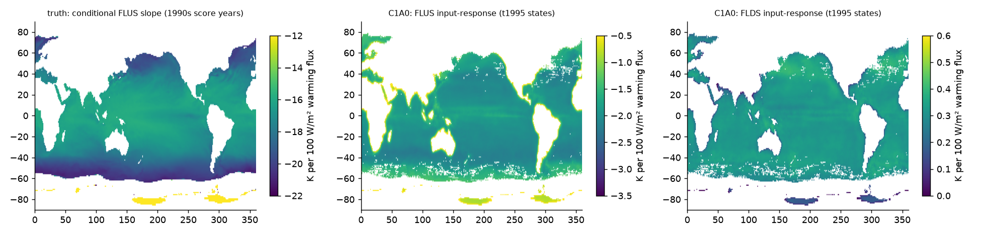
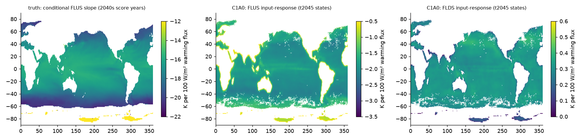
Interpretation (open). The data contain the leak in its strongest form, so a model that fit the linear truth relation would answer ~17 K per 100 W/m² to FLUS and ~0 to everything else. C1A0 does neither. One candidate: its ocean was fine-tuned in coupled mode (E35-CFT), where FLUS comes from the atmosphere driven by the ocean's start-of-window SST, so the leak is absent there. The replication across checkpoints (E11-FT = the same ocean before coupled fine-tuning; E11 seeds; E12–E16) tests this directly.
Reproduce
python idea1_flus/f1_extract.py 1995 1996 1997 1998 1999 2040 2041 2042 2043 2044 2045 2046 2047 2048 2049 1985 1986 1987 1988 1989
python idea1_flus/f1_analyze.py
python -m hc.evaluate data/states/t1995 --start 1995-01-01 --steps 73 --capture --atm-spectra && python -m hc.meta data/states/t1995
python -m hc.evaluate data/states/t2045 --start 2045-01-01 --steps 73 --capture --atm-spectra && python -m hc.meta data/states/t2045
python idea1_flus/f1_model_compare.py data/states/t1995 1990s t1995
python idea1_flus/f1_model_compare.py data/states/t2045 2040s t2045
Results: f1.json f1_compare_t1995.json f1_compare_t2045.json
F2 · Where the response goes: exact patching below “skip.0 + layer 0”
Layer 0 is the network's only reader of the input: skip_module (1×1 conv, no norm) + convblock (3×3 conv → InstanceNorm → GELU → 3×3 conv → InstanceNorm → GELU → 1×1 conv). Its output feeds the full-resolution skip (skip.0) and the deep path. Exact clean→corrupted patching over the factorial {skip_module, convblock, convblock with clean InstanceNorm statistics} × {skip.0, deep}; perturbations: each flux, sst, sst + 0–20 m temperature; uniform open-ocean and 10×10° boxes on the preregistered lattice.
t1995|uniform
| perturbation | slope (K/100 W/m²; K/K for sst) | /FLDS | skip.0 only | deep only | skip_module only | convblock only | convblock, IN frozen |
|---|---|---|---|---|---|---|---|
| FLUS | -1.829 [-1.845, -1.808] | -5.79 | 0.86 / 0.86 | 0.14 / 0.14 | 0.52 / 0.50 | 0.48 / 0.50 | 0.94 / 1.19 |
| FLDS | +0.316 [+0.309, +0.322] | +1.00 | 0.75 / 0.74 | 0.25 / 0.26 | 0.78 / 0.77 | 0.22 / 0.23 | 0.55 / 0.55 |
| FSNS | +0.286 [+0.282, +0.289] | +0.91 | 1.08 / 1.06 | -0.08 / -0.06 | 1.09 / 0.97 | -0.09 / 0.03 | -0.29 / -0.14 |
| LHFLX | +0.073 [+0.068, +0.080] | +0.23 | 1.36 / 1.01 | -0.35 / -0.01 | 0.29 / 0.30 | 0.71 / 0.71 | 1.81 / 0.89 |
| SHFLX | +0.129 [+0.125, +0.133] | +0.41 | 0.57 / 0.63 | 0.43 / 0.37 | 1.83 / 1.16 | -0.83 / -0.16 | -2.30 / -1.00 |
| sstT0 | +0.499 [+0.498, +0.500] | – | 0.89 / 0.89 | 0.11 / 0.11 | 1.00 / 0.99 | 0.00 / 0.01 | -0.04 / -0.03 |
| sst | +0.222 [+0.222, +0.223] | – | 0.89 / 0.89 | 0.11 / 0.11 | 1.00 / 1.00 | -0.00 / 0.00 | -0.06 / -0.06 |
t1995|box
| perturbation | slope (K/100 W/m²; K/K for sst) | /FLDS | skip.0 only | deep only | skip_module only | convblock only | convblock, IN frozen |
|---|---|---|---|---|---|---|---|
| FLUS | -2.572 [-2.971, -2.271] | -7.84 | 0.91 / 0.91 | 0.09 / 0.09 | 0.35 / 0.30 | 0.65 / 0.70 | 0.65 / 0.70 |
| FLDS | +0.332 [+0.246, +0.443] | +1.00 | 0.93 / 0.92 | 0.07 / 0.08 | 0.52 / 0.50 | 0.48 / 0.50 | 0.49 / 0.50 |
| FSNS | +0.255 [+0.164, +0.352] | +0.77 | 0.99 / 0.95 | 0.01 / 0.06 | 1.31 / 0.67 | -0.31 / 0.33 | -0.31 / 0.33 |
| LHFLX | +0.115 [-0.001, +0.245] | +0.33 | 0.89 / 0.94 | 0.11 / 0.06 | 0.05 / 0.28 | 0.95 / 0.72 | 0.95 / 0.72 |
| SHFLX | -0.132 [-0.269, -0.027] | -0.40 | 1.12 / 0.90 | -0.13 / 0.10 | -1.91 / -0.40 | 2.90 / 1.40 | 2.91 / 1.40 |
| sstT0 | +0.468 [+0.419, +0.516] | – | 0.90 / 0.89 | 0.10 / 0.11 | 1.05 / 1.05 | -0.05 / -0.05 | -0.05 / -0.05 |
| sst | +0.205 [+0.183, +0.228] | – | 0.89 / 0.89 | 0.11 / 0.11 | 1.08 / 1.07 | -0.08 / -0.07 | -0.08 / -0.07 |
t2045|uniform
| perturbation | slope (K/100 W/m²; K/K for sst) | /FLDS | skip.0 only | deep only | skip_module only | convblock only | convblock, IN frozen |
|---|---|---|---|---|---|---|---|
| FLUS | -1.801 [-1.822, -1.786] | -5.77 | 0.86 / 0.85 | 0.15 / 0.15 | 0.53 / 0.51 | 0.47 / 0.49 | 0.94 / 1.22 |
| FLDS | +0.312 [+0.306, +0.317] | +1.00 | 0.75 / 0.74 | 0.25 / 0.26 | 0.79 / 0.78 | 0.21 / 0.22 | 0.55 / 0.56 |
| FSNS | +0.289 [+0.285, +0.293] | +0.93 | 1.07 / 1.05 | -0.07 / -0.05 | 1.09 / 0.96 | -0.09 / 0.04 | -0.29 / -0.13 |
| LHFLX | +0.068 [+0.064, +0.076] | +0.22 | 1.41 / 1.01 | -0.40 / -0.00 | 0.28 / 0.29 | 0.72 / 0.71 | 1.92 / 0.88 |
| SHFLX | +0.133 [+0.126, +0.139] | +0.43 | 0.58 / 0.64 | 0.42 / 0.36 | 1.77 / 1.14 | -0.77 / -0.14 | -2.24 / -0.99 |
| sstT0 | +0.500 [+0.498, +0.502] | – | 0.89 / 0.89 | 0.11 / 0.11 | 0.99 / 0.99 | 0.01 / 0.01 | -0.04 / -0.03 |
| sst | +0.223 [+0.222, +0.224] | – | 0.89 / 0.89 | 0.11 / 0.11 | 1.00 / 1.00 | 0.00 / 0.00 | -0.06 / -0.06 |
t2045|box
| perturbation | slope (K/100 W/m²; K/K for sst) | /FLDS | skip.0 only | deep only | skip_module only | convblock only | convblock, IN frozen |
|---|---|---|---|---|---|---|---|
| FLUS | -2.582 [-2.947, -2.226] | -7.82 | 0.91 / 0.90 | 0.09 / 0.09 | 0.35 / 0.30 | 0.65 / 0.70 | 0.65 / 0.70 |
| FLDS | +0.334 [+0.247, +0.458] | +1.00 | 0.93 / 0.91 | 0.07 / 0.09 | 0.52 / 0.50 | 0.48 / 0.50 | 0.48 / 0.50 |
| FSNS | +0.256 [+0.170, +0.348] | +0.77 | 0.98 / 0.94 | 0.01 / 0.06 | 1.31 / 0.66 | -0.31 / 0.34 | -0.31 / 0.34 |
| LHFLX | +0.117 [+0.018, +0.251] | +0.34 | 0.89 / 0.94 | 0.10 / 0.06 | -0.46 / 0.27 | 1.46 / 0.73 | 1.47 / 0.73 |
| SHFLX | -0.140 [-0.239, -0.028] | -0.42 | 1.10 / 0.90 | -0.11 / 0.09 | -1.73 / -0.40 | 2.72 / 1.40 | 2.73 / 1.40 |
| sstT0 | +0.467 [+0.417, +0.530] | – | 0.90 / 0.89 | 0.10 / 0.11 | 1.06 / 1.05 | -0.06 / -0.05 | -0.06 / -0.05 |
| sst | +0.204 [+0.179, +0.236] | – | 0.89 / 0.89 | 0.11 / 0.11 | 1.08 / 1.08 | -0.08 / -0.08 | -0.08 / -0.08 |
samudra Patchable adapter, EdgePatch semantics) gives skip.0 share 0.854 on 7 states of 2045 (localize.py: 0.86)Cells: perturbed-area-mean share / projection share. Because the network is near-linear in dQ, sufficiency = necessity and skip.0 + deep ≈ 1: one result, not converging lines.
Reproduce
python idea1_flus/localize.py data/states/t1995 t1995 4
python idea1_flus/localize.py data/states/t2045 t2045 4
python idea1_flus/localize_summary.py t1995 t2045
Results: localize_summary_t1995.json localize_summary_t2045.json
F3 · Can FLUS be removed without breaking FLDS/FSNS?
| shift | arm | FLUS × | FLDS × | FSNS × | LHFLX × | SHFLX × | PREREG success |
|---|---|---|---|---|---|---|---|
| uniform | greedy10 | 0.51 | 0.54 | 0.29 | 5.56 | -0.00 | no |
| uniform | greedy32 | 0.08 | -0.06 | 0.79 | 6.24 | -1.06 | no |
| uniform | deleak_input | -0.00 | 1.00 | 1.02 | 0.98 | 1.02 | yes |
| uniform | random10 ×20 | 0.97 [0.85, 1.02] | 0 successes | ||||
| uniform | random32 ×20 | 0.87 [0.75, 1.01] | 0 successes | ||||
| box | greedy10 | 0.51 | 0.33 | 0.28 | 4.02 | 1.07 | no |
| box | greedy32 | 0.08 | -0.15 | 0.90 | 4.36 | 1.58 | no |
| box | deleak_input | -0.00 | 1.10 | 0.88 | 1.15 | 1.67 | yes |
| box | random10 ×20 | 0.97 [0.85, 1.04] | 0 successes | ||||
| box | random32 ×20 | 0.88 [0.75, 1.04] | 0 successes |
Ratios are ablated / unablated slope per state, averaged (LHFLX ratios are unstable because its unablated slope is small). Greedy channels at layer 0: 254, 51, 203, 179, 33, 14, 256, 127, 30, 57 … (channel 254 first, as on the laptop). Greedy curve on fit states: 10 channels 0.48, 32 channels 0.91 of the FLUS response.
Reproduce
python idea1_flus/ablate.py l0 data/states/ic1985,data/states/t1995 data/states/t2045 v1
python idea1_flus/ablate_summary.py ablate_l0_v1
Results: ablate_l0_v1_summary.json
Replication across checkpoints
| checkpoint | training | FLUS | FLDS | FSNS | LHFLX | SHFLX | FLUS box | thermometer area | shortcut? |
|---|---|---|---|---|---|---|---|---|---|
| E11-FT_S02 | ocean-only + fine-tune (leaky FLUS) | -7.07 | +0.52 | +0.08 | -0.56 | +0.33 | -9.08 | 0.989 | yes |
| E11-FT_S01 | ocean-only + fine-tune (leaky FLUS) | -6.97 | +0.26 | +0.07 | -0.51 | +0.34 | -8.84 | 0.988 | yes |
| E11-FT_S03 | ocean-only + fine-tune (leaky FLUS) | -6.85 | +0.35 | +0.06 | -0.49 | +0.32 | -8.79 | 0.988 | yes |
| E12_W1 | ocean-only, loss-weight variant | -5.50 | +0.22 | +0.15 | -0.14 | +0.14 | -7.87 | 0.992 | yes |
| E13_W2 | ocean-only, loss-weight variant | -5.24 | +0.16 | +0.09 | -0.21 | +0.23 | -7.60 | 0.989 | yes |
| E11_S02 | ocean-only, truth-forced (leaky FLUS) | -4.23 | +0.43 | +0.19 | -0.21 | +0.14 | -5.81 | 0.996 | yes |
| E14_W4 | ocean-only, loss-weight variant | -4.14 | +0.13 | +0.17 | -0.10 | +0.16 | -6.09 | 0.995 | yes |
| E16_W3 | ocean-only, loss-weight variant | -4.05 | +0.18 | +0.19 | -0.16 | +0.23 | -5.97 | 0.996 | yes |
| E11_S03 | ocean-only, truth-forced (leaky FLUS) | -4.03 | +0.28 | +0.18 | -0.05 | +0.07 | -5.60 | 0.993 | yes |
| E11_S01 | ocean-only, truth-forced (leaky FLUS) | -3.99 | +0.15 | +0.17 | -0.17 | +0.17 | -5.90 | 0.994 | yes |
| E30-CFT_S01 | coupled fine-tune (C0A0 family seed) | -2.49 | +0.28 | +0.26 | +0.03 | +0.22 | -3.45 | 0.995 | yes |
| E30-CFT_S02 | coupled fine-tune (C0A0 family seed) | -2.02 | +0.55 | +0.30 | +0.08 | +0.17 | -2.81 | 0.998 | yes |
| C1A1 | coupled fine-tune (release) | -1.98 | +0.31 | +0.28 | +0.07 | +0.17 | -2.76 | 0.997 | yes |
| E31-CFT_S02 | coupled fine-tune (C1A1 family seed) | -1.98 | +0.56 | +0.33 | +0.08 | +0.15 | -2.74 | 0.998 | yes |
| E31-CFT_S03 | coupled fine-tune (C1A1 family seed) | -1.87 | +0.44 | +0.31 | +0.03 | +0.33 | -2.73 | 0.996 | yes |
| C1A0 | coupled fine-tune (release) | -1.84 | +0.32 | +0.29 | +0.08 | +0.13 | -2.57 | 0.997 | yes |
| C0A0 | coupled fine-tune (release) | -1.71 | +0.43 | +0.31 | +0.05 | +0.24 | -2.51 | 0.997 | yes |
Reproduce
python idea1_flus/replicate.py C1A0=... E11-FT_S01=... (see slurm/queue scripts 08_replicate_*.sh)
Results: replicate_C1A0.json replicate_E11-FT_S02.json replicate_E12_W1.json replicate_E30-CFT_S01.json
Idea 2 · Do explanations keep the emulator's real errors?
Plan (preregistered, Phase 2). One-step forecasts from truth states (atmosphere 6 h, 4 seeds; ocean 5 days, truth-forced). Error = model − E3SM. Tolerance τ = max(2 × same-seed SD, 1% of spatial SD), sweep k ∈ {1, 2, 3}. Explanations: ocean skip.0-only, atmosphere blocks-only / big-skip-only (corrector in/out), PCA-k / SAE at SFNO blocks. Scores: A_ok, A_err, three-way split (reproduces / corrects / other), scalar-offset and per-component-gain controls, empty-explanation and seed-ceiling anchors, block bootstrap.
Starter result (hackathon track T2; not a finished result)
One-step forecasts from 12 truth states (fit: 1996, 2042; score: 4 dates of 2047), 4 seeds, pre-corrector, τ = max(2σ_seed, 1% spatial SD). Cells: A_ok / A_err.
| variable | error area | seed ceiling | empty (PCA-0) | PCA-8 L7 | PCA-32 L7 | PCA-128 L7 | scalar offset | affine persistence |
|---|---|---|---|---|---|---|---|---|
| TS | 0.33 | 0.83 / 0.80 | 0.23 / 0.17 | 0.32 / 0.25 | 0.50 / 0.39 | 0.88 / 0.77 | 0.29 / 0.19 | 0.33 / 0.16 |
| T_7 | 0.21 | 0.83 / 0.79 | 0.22 / 0.16 | 0.30 / 0.22 | 0.65 / 0.52 | 0.95 / 0.88 | 0.41 / 0.28 | 0.39 / 0.28 |
| U_7 | 0.25 | 0.83 / 0.78 | 0.19 / 0.13 | 0.37 / 0.26 | 0.58 / 0.43 | 0.91 / 0.78 | 0.33 / 0.23 | 0.32 / 0.23 |
| PS | 1.00 | – | – | – | – | – | – | – |
| surface_precipitation_rate | 0.68 | 0.82 / 0.82 | 0.31 / 0.28 | 0.38 / 0.34 | 0.65 / 0.62 | 0.84 / 0.81 | – | – |
| FLUT | 0.25 | 0.83 / 0.77 | 0.30 / 0.22 | 0.40 / 0.31 | 0.65 / 0.51 | 0.94 / 0.87 | – | – |
| FSUTOA | 0.36 | 0.82 / 0.80 | 0.31 / 0.18 | 0.30 / 0.21 | 0.40 / 0.25 | 0.74 / 0.56 | – | – |
Latent explanations beat the output-level controls by a wide margin; PCA-128 at block 7 reaches the seed ceiling for T_7 and FLUT. PS is 'error' everywhere and precipitation on 68% because this is pre-corrector output: the corrector column is the first thing to add. No bootstrap; 4 score dates.
Idea 3 · How much of each spatial scale survives one step?
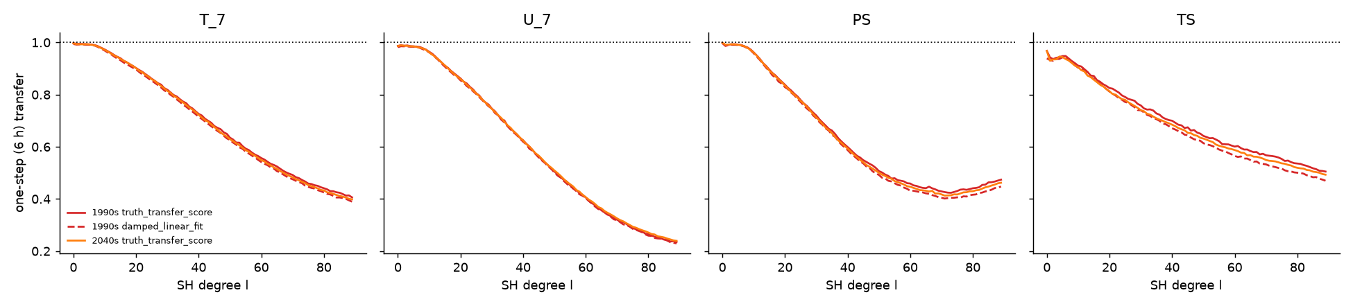
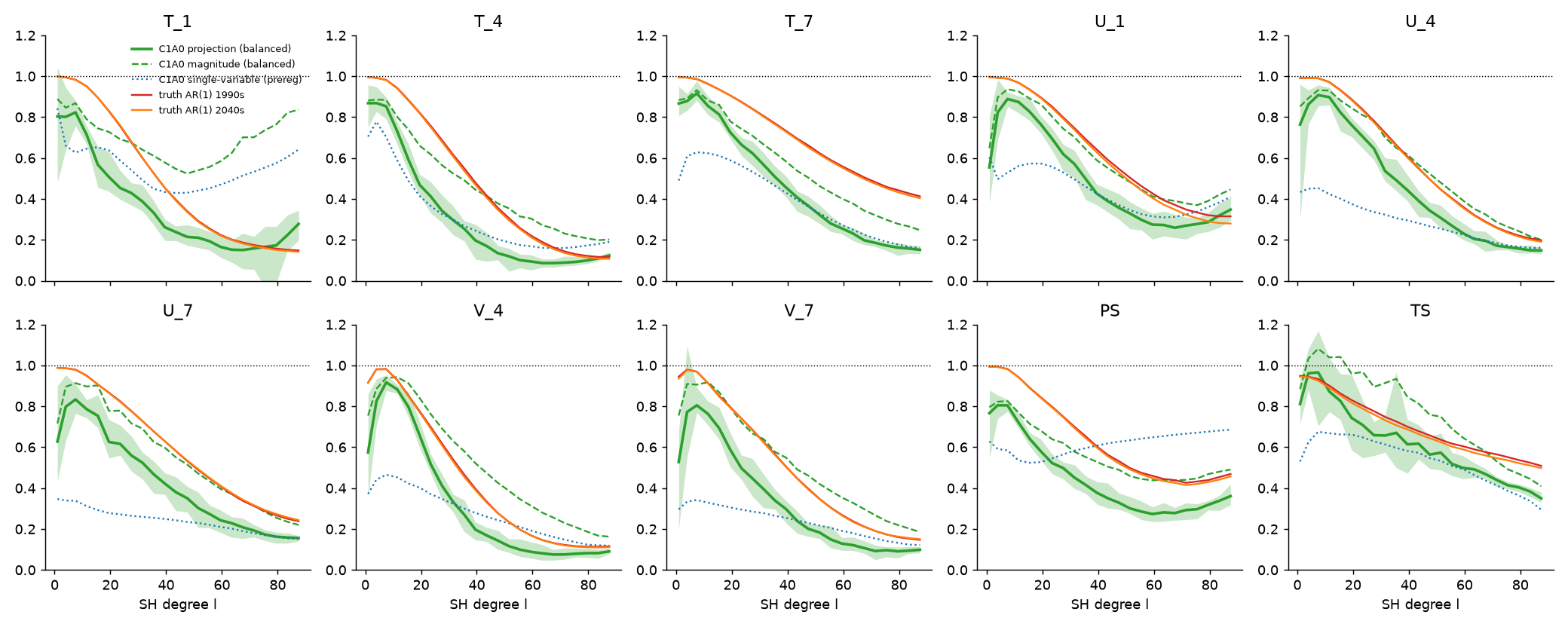
Method. JVP of the 6-hour atmosphere network (pre-corrector) at 12 truth states (Jan/Apr/Jul/Oct × 1996, 2042, 2047) × 3 noise draws, noise held fixed by passing our own draw to the conditional model. Probes: band-limited random fields (flat power over the band, 8 per band, physical units: K, m/s, Pa); gain(band) = √(output power in band / input power in band). Baselines: persistence (1); E3SM's own per-degree one-step AR(1) transfer of anomalies (score years) and the damped-linear fit (fit years). These two are the same statistic on different years, a restatement, shown to bound sampling noise.
Reproduce
python idea3_gain/truth_transfer.py coeffs 1995 1996 1997 1998 1999 2040 2041 2042 2043 2044 2045 2046 2047 2048 2049
python idea3_gain/truth_transfer.py transfer
Results: truth_transfer.json
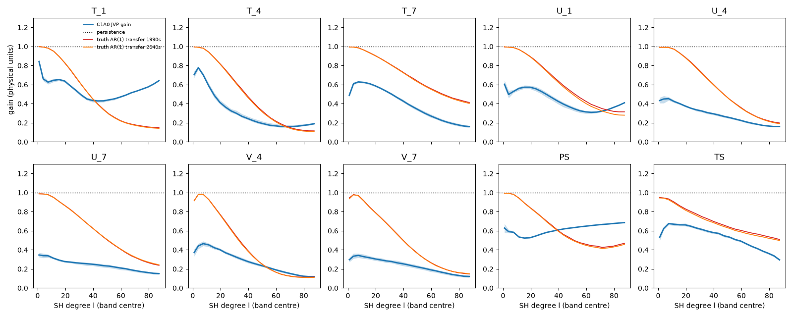
Linearity (finite difference / JVP, per probe): PS|band0-2|eps0.01: 0.998–1.001; PS|band0-2|eps0.1: 0.974–1.005; PS|band14-17|eps0.01: 1.000–1.001; PS|band14-17|eps0.1: 0.994–1.005; PS|band30-33|eps0.01: 1.000–1.000; PS|band30-33|eps0.1: 0.998–1.002; PS|band46-49|eps0.01: 1.000–1.000; PS|band46-49|eps0.1: 0.997–1.001; PS|band62-65|eps0.01: 1.000–1.000; PS|band62-65|eps0.1: 1.000–1.000; PS|band78-81|eps0.01: 1.000–1.000; PS|band78-81|eps0.1: 1.000–1.000; T_7|band0-2|eps0.01: 0.984–1.006; T_7|band0-2|eps0.1: 0.905–1.131; T_7|band14-17|eps0.01: 0.998–1.000; T_7|band14-17|eps0.1: 0.987–1.005; T_7|band30-33|eps0.01: 1.000–1.000; T_7|band30-33|eps0.1: 0.999–1.001; T_7|band46-49|eps0.01: 1.000–1.000; T_7|band46-49|eps0.1: 0.999–1.000; T_7|band62-65|eps0.01: 1.000–1.000; T_7|band62-65|eps0.1: 1.000–1.000; T_7|band78-81|eps0.01: 1.000–1.004; T_7|band78-81|eps0.1: 1.000–1.000; U_7|band0-2|eps0.01: 0.999–1.000; U_7|band0-2|eps0.1: 0.993–1.005; U_7|band14-17|eps0.01: 1.000–1.000; U_7|band14-17|eps0.1: 0.999–1.001; U_7|band30-33|eps0.01: 1.000–1.000; U_7|band30-33|eps0.1: 1.000–1.000; U_7|band46-49|eps0.01: 1.000–1.000; U_7|band46-49|eps0.1: 1.000–1.000; U_7|band62-65|eps0.01: 1.000–1.003; U_7|band62-65|eps0.1: 1.000–1.000; U_7|band78-81|eps0.01: 1.000–1.010; U_7|band78-81|eps0.1: 1.000–1.000.
Reproduce
python -m hc.evaluate data/states/atm12 --steps 1 --capture-atm 1 --no-ocn-pred --capture --start 1996-01-16 ... (12 dates)
python idea3_gain/gain_atm.py data/states/atm12 a 0 1 2  # ... b 3 4 5, c 6 7 8, d 9 10 11
python idea3_gain/gain_summary.py a b c d
Results: gain_atm_summary.json
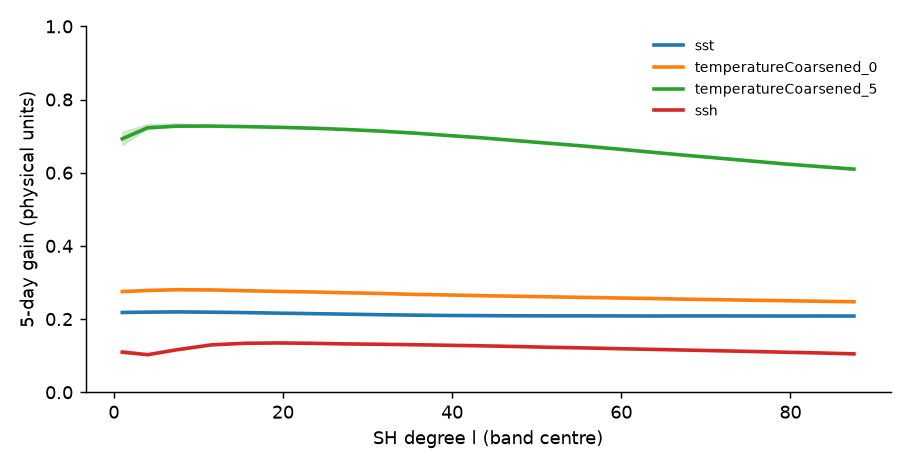
Ocean, 5-day step
Balanced probes (exploratory, PREREG change log 2026-11-20)
Reproduce
python -m hc.evaluate data/states/atm12m5 --steps 1 --capture-atm 1 --no-ocn-pred --start 1996-01-11 ... (12 dates − 5 d)
python idea3_gain/gain_atm_bal.py data/states/atm12 data/states/atm12m5 v2
Results: gain_atm_bal_v2.json
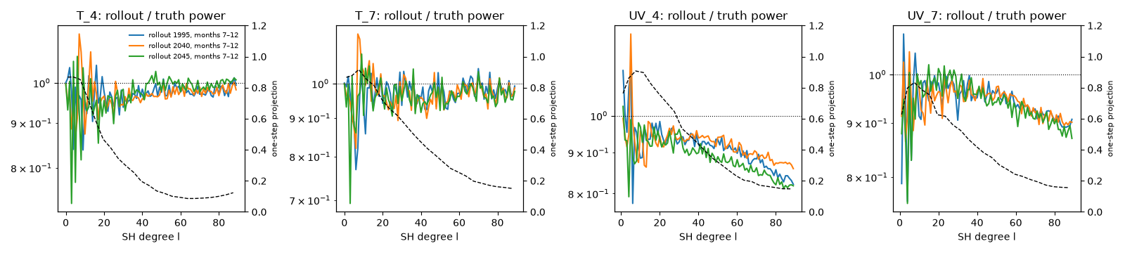
Rollout spectra (starter, track T3)
Pending: other checkpoints; ViT comparison
Numbers that are restatements of one another
- F1 (b) FLUS coefficient and its Frisch–Waugh version (agree to 5e-9).
- Truth one-step transfer (score years) and the damped-linear AR(1) fit (fit years): one statistic, two year sets.
- Edge-patching sufficiency and necessity, and skip.0 + deep ≈ 1, under a near-linear response.
- The laptop's zero-net violation, Eq. 10 M and joint M all follow from the FLUS/FLDS ratio (PLAN Sec. 2.3).
For participants and their agents
Start with HACKATHON.md: setup in ~20 min, what is ready, six open tracks, and a prompt to hand your agent.
- Code: https://github.com/mahf708/samudrace-circuits · data products (held-out states with truth targets, truth extracts, results): https://huggingface.co/datasets/mahf708/samudrace-circuits
- REPORT.md: findings with controls and caveats; verified / narrowed / open per idea
- exege
samudraadapter (Patchable + EdgeGradients): mahf708/exege#12 - AGENTS.md: where everything is, the exact libraries, pitfalls we hit
- manifest.json: every claim on this page with value, verdict, control, caveat, source JSON, script and command
- PREREG.md (fixed before results, with change log) · INVENTORY.md
Updated 2026-11-20 06:57 . Every number links to its JSON under “Reproduce”; machine-readable: manifest.json.