Making Sparse Gaussian Elimination Scalable by Static Pivoting
Xiaoye S. Li

NERSC, Lawrence Berkeley National Lab
1 Cyclotron Rd, MS 50F
Berkeley, CA 94720.
xiaoye@nersc.gov
http://www.nersc.gov/~xiaoye
James W. Demmel

Computer Science Division
University of California
Berkeley, CA 94720.
demmel@cs.berkeley.edu
http://www.cs.berkeley.edu/~demmel
Abstract:
-
We propose several techniques as alternatives to partial pivoting
to stabilize sparse Gaussian elimination. From numerical experiments
we demonstrate that for a wide range of problems the new method
is as stable as partial pivoting.
The main advantage of the new method
over partial pivoting is that it permits a priori
determination of data structures and communication pattern
for Gaussian elimination, which makes it more scalable on distributed
memory machines. Based on this a priori knowledge,
we design highly parallel algorithms for both sparse Gaussian elimination
and triangular solve and we show that they are suitable for large-scale
distributed memory machines.
- Keywords:
- sparse unsymmetric linear systems, static pivoting,
iterative refinement, MPI, 2-D matrix decomposition.
In our earlier work [8, 9, 22],
we developed new algorithms to solve unsymmetric sparse linear
systems using Gaussian elimination with partial pivoting (GEPP).
The new algorithms are highly efficient on workstations with deep
memory hierarchies and shared memory parallel machines with a
modest number of processors. The portable implementations of these
algorithms appear in the software packages SuperLU (serial) and
SuperLU_MT (multithreaded), which are publically available
on Netlib [10]. These are among the fastest available
codes for this problem.
Our shared memory GEPP algorithm relies on the fine-grained memory access
and synchronization that shared memory provides to manage the
data structures needed as fill-in is created dynamically,
to discover which columns depend on which other columns symbolically,
and to use a centralized task queue for scheduling and load
balancing. The reason we have to perform all these dynamically
is that the computational graph does not unfold until runtime.
(This is in contrast to Cholesky, where any pivot order is
numerically stable.)
However, these techniques are too expensive on distributed memory
machines. Instead, for distributed memory machines, we propose
to not pivot dynamically, and so enable static data structure
optimization, graph manipulation and load balancing
(as with Cholesky [20, 25])
and yet remain numerically stable.
We will retain numerical stability by a variety of techniques:
pre-pivoting large elements to the diagonal, iterative refinement,
using extra precision when needed, and allowing
low rank modifications with corrections at the end.
In Section 2 we show the promise of the proposed method
from numeric experiments. We call our algorithm GESP for
Gaussian elimination with static pivoting.
In Section 3, we present an MPI implementation of the
distributed algorithms for LU factorization and triangular solve.
Both algorithms use an elaborate 2-D (nonuniform)
block-cyclic data distribution. Initial results demonstrated
good scalability and a factorization rate exceeding 8 Gflops
on a 512 node Cray T3E.
Traditionally, partial pivoting is used
to control the element growth during Gaussian elimination,
making the algorithm numerically stable in practice .
However partial pivoting is not the only way to control element growth;
there are a variety of alternative techniques.
In this section we present these alternatives, and
show by experiments that appropriate combinations of them
can effectively stabilize Gaussian elimination.
Furthermore, these techniques are usually inexpensive compared
to the overall solution cost, especially for large problems.

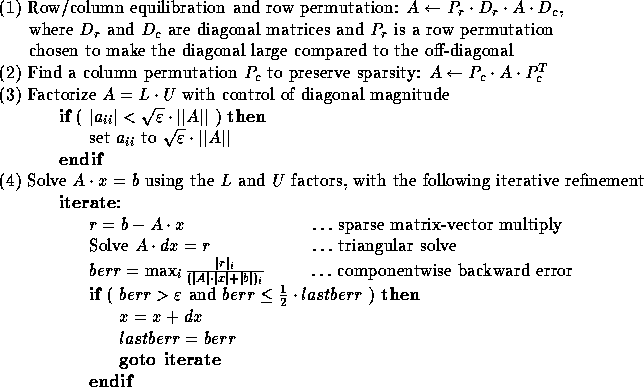
Figure 1: The outline of the new GESP algorithm.
In Figure 1 we sketch our GESP algorithm that
incorporates some of the techniques we considered.
To motivate step (1), recall that a diagonally dominant
matrix is one where each diagonal entry  is larger in
magnitude than the sum of magnitudes of the off-diagonal entries in its
row (
  ) or column (
  ).
It is known that choosing the diagonal pivots ensures
stability for such matrices [7, 19].
So we expect that if each diagonal entry
can somehow be made larger relative to the off-diagonals in its row
or column, then diagonal pivoting will be more stable.
The purpose of step (1) is to choose diagonal matrices
 and
and  and permutation
  to make each
  larger in this sense.
We have experimented with a number of alternative heuristic algorithms
for step (1) [13]. All depend on the following graph
representation of an  sparse matrix A: it is represented
as an undirected weighted bipartite graph with one vertex for each row,
one vertex for each column, and an edge with appropriate weight
connecting row vertex i
to column vertex j for each nonzero entry
  . Finding a permutation
 that puts large entries on the diagonal can thus be transformed into
a weighted bipartite matching problem on this graph. The diagonal scale
matrices
  and
and  can be chosen independently, to make each row
and each column of
  have largest entries equal to 1 in magnitude
(using the algorithm in LAPACK subroutine DGEEQU [3]).
Then there are algorithms in [13] that choose
  to
maximize different properties of the diagonal of
  , such as
the smallest magnitude of any diagonal entry, or the sum or product
of magnitudes. But the best algorithm in practice seems to be the one
in [13] that picks
  ,
,  and
and  simultaneously
so that each diagonal entry of
  is
is  ,
each off-diagonal entry is bounded by 1 in magnitude,
and the product of the diagonal entries is maximized.
We will report results for this algorithm only.
The worst case serial complexity of this algorithm is
 , where nnz(A) is the
number of nonzeros in A.
In practice it is much faster; actual timings appear later.
Step (2) is not new and is needed in both SuperLU and
SuperLU_MT [10].
The column permutation  can be obtained from any fill-reducing
heuristic. For now, we use the minimum degree ordering algorithm [23]
on the structure of
  . In the future, we will
use the approximate minimum degree column ordering algorithm
by Davis et. al. [6] which is faster and requires
less memory since it does not explicitly form
  .
We can also use nested dissection on
  or
or  [17].
Note that we also apply
  to the rows of A to ensure that the
large diagonal entries obtained from Step (1) remain on the diagonal.
In step (3), we simply set any tiny pivots encountered during elimination to
 ,
where
  is machine precision. This is equivalent to a small
(half precision) perturbation to the original problem, and trades off
some numerical stability for the ability to keep pivots from
getting too small.
In step (4), we perform a few steps of iterative refinement if
the solution is not accurate enough, which also corrects for the
 perturbations in step (3).
The termination criterion
is based on the componentwise backward error berr [7].
The condition
  means that the computed solution
is the exact solution of a slightly different sparse linear system
 where each nonzero entry
  has been changed by at most one
unit in its last place, and the zero entries are left unchanged;
thus one can say that the answer is as accurate as the data deserves.
We terminate the iteration when the backward error berr is
smaller than machine epsilon, or when it does not decrease by at least a factor
of two compared with the previous iteration. The second test
is to avoid possible stagnation. (Figure 5 shows that berr is
always small.)
In this subsection, we illustrate the numerical stability and runtime
of our GESP algorithm on 53 unsymmetric matrices from a wide variety
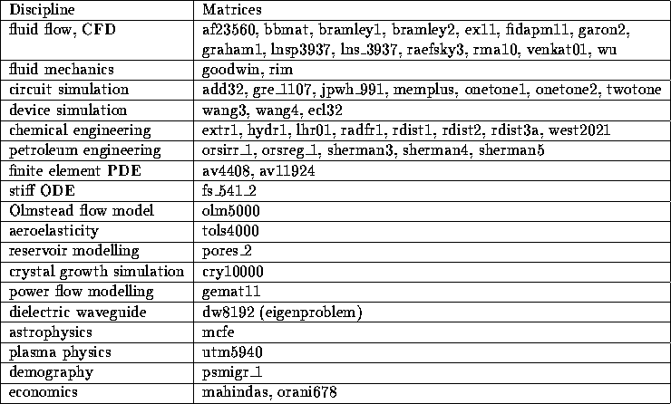
of applications. The application domains of the matrices
are given in Table 1.
Most of them, except for two (ECL32, WU), can be obtained from the
Harwell-Boeing Collection [14] and the collection of
Davis [5]. Matrix ECL32 was provided by Jagesh Sanghavi from
EECS Department of UC Berkeley. Matrix WU was provided by Yushu Wu from
Earth Sciences Division of Lawrence Berkeley National Laboratory.
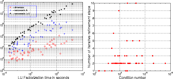
Figure 2 plots the dimension, nnz(A), and
nnz(L+U), i.e. the number of nonzeros in the L and U factors
(the fill-in).
The matrices are sorted in increasing
order of the factorization time. The matrices of most interest for
parallelization are the ones that take the most time, i.e. the
ones on the right of this graph.
From the figure it is clear that the
matrices large in dimension and number of nonzeros also require more time
to factorize.
The timing results reported in this subsection are obtained on
an SGI ONYX2 machine running IRIX 6.4.
The system has 8 195 MHz MIPS R10000
processors and 5120 Mbytes main memory. We only use a single processor,
since we are mainly interested in numerical accuracy.
Parallel runtimes are reported in section 3.
Detailed performance results from this section in tabular format
are available at
http://www.nersc.gov/  xiaoye/SC98/.

Table 1: Test matrices and their disciplines.
Among the 53 matrices, most would get wrong answers or fail completely
(via division by a zero pivot) without any pivoting or other precautions.
22 matrices contain zeros on the diagonal to begin with which remain zero
during elimination, and 5 more create zeros on the diagonal during elimination.
Therefore, not pivoting at all would fail completely on these 27 matrices.
Most of the other 26 matrices would get unacceptably large errors due
to pivot growth.
For our experiment, the right-hand side vector is generated so that
the true solution  is a vector of all ones.
IEEE double precision is used as the working precision, with
machine epsilon
  .
Figure 3 shows the number of iterations taken in the iterative
refinement step. Most matrices terminate the iteration with
no more than 3 steps. 5 matrices require 1 step, 31 matrices
require 2 steps, 9 matrices require 3 steps, and 8 matrices
require more than 3 steps.
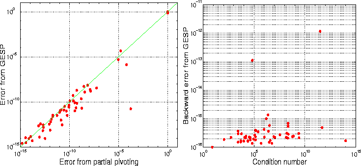
For each matrix, we present two error metrics, in Figure 4
and Figure 5, to assess the accuracy and stability of GESP.
Figure 4 plots the error from GESP versus the error from GEPP
(as implemented in SuperLU) for each matrix:
A red dot on the green diagonal means the two errors were
the same, a red dot below the diagonal means GESP is more accurate, and
a red dot above means GEPP is more accurate.
Figure 4 shows that the error of GESP
is at most a little larger, and usually smaller (37 times out of 53),
than the error from GEPP.
Figure 5 shows that the
componentwise backward error [7] is also small,
usually near machine epsilon, and never larger than
  .
.
Although the combination of the techniques in steps (1) and (3)
in Figure 1 works well for most matrices,
we found a few matrices for which other
combinations are better. For example, for FIDAPM11, JPWH_991
and ORSIRR_1, the errors are large unless we omit  from step (1).
For EX11 and RADRF1, we cannot replace tiny pivots by
 (in step (3)).
Therefore, in the software, we provide a flexible interface so
the user is able to turn on or off any of these options.

Figure 2: Characteristics of the matrices.
Figure 3: Iterative refinement steps in GESP.

Figure 4: The error  .
Figure 5: The backward error
 .
.

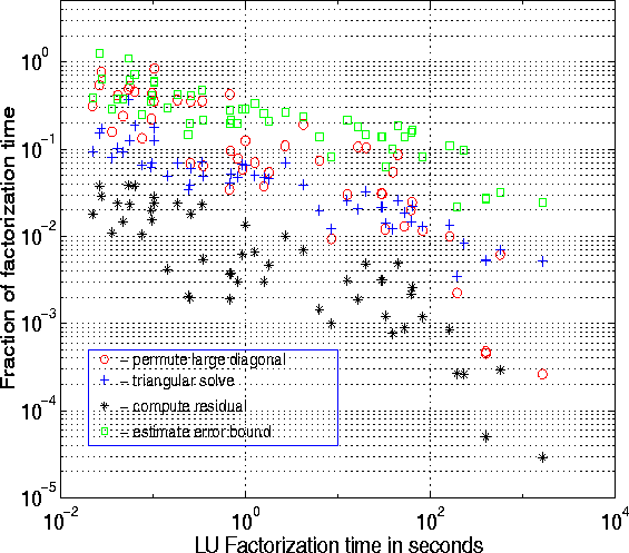
Figure 6: The times to factorize, solve, permute large diagonal, compute
residual and estimate error bound, on a 195 MHz MIPS R10000.
We now evaluate the cost of each step in GESP Figure 1.
This is done with respect to the serial implementation,
since we have only parallelized the numerical phases of the
algorithm (steps (3) and (4)), which are the most time-consuming.
In particular, for large enough matrices, the LU factorization
in step (3) dominates all the other steps, so we will measure
the times of each step with respect to step (3).
Simple equilibration in step (1) (computing  and
and  using
the algorithm in DGEEQU from LAPACK)
is usually negligible and is easy to parallelize.
Both row and column permutation algorithms in steps (1) and (2)
(computing
  and
and  ) are not easy to parallelize
(their parallelization is future work).
Fortunately, their memory requirement is just
O(nnz(A)) [6, 13],
whereas the memory requirement for L and U
factors grows superlinearly in nnz(A), so in the meantime
we can run them on a single processor.
Figure 6 shows the fraction of time spent finding
 in step (1) using the
algorithm in [13], as a fraction of the factorization time.
The time is significant for small problems, but drops to 1% to 10%
for large matrices requiring a long time to factor,
the problems of most interest on parallel machines.
The time to find a sparsity-preserving ordering  in step (2)
is very much matrix dependent.
It is usually cheaper than factorization,
although there exist matrices for which the ordering is more expensive.
Nevertheless, in applications where we repeatedly solve a
system of equations with the same nonzero pattern but different
values, the ordering algorithm needs to be run only once, and its
cost can be amortized over all the factorizations.
We plan to replace this part of the algorithm with something
faster, as outlined in Section 2.1.
As can be seen in Figure 6, computing the residual
(sparse matrix-vector multiplication  )
is cheaper than a triangular solve (
  ),
and both take a small fraction of the factorization time.
For large matrices the solve time is often less than 5%
of the factorization time. Both algorithms have been parallelized
(see section 3 for parallel performance data).
Finally, our code has the ability to estimate a forward error bound
for the true error  .
This is by far the most expensive step after factorization.
(For small matrices, it can be more expensive than factorization,
since it requires multiple triangular solves.)
Therefore, we will do this only when the user asks for it.
In this section, we describe our design, implementation and the
performance of the distributed algorithms for two main steps of
the GESP method, sparse LU factorization (step (3)) and sparse
triangular solve (used in step (4)).
Our implementation uses MPI [26]
to communicate data, and so is highly portable.
We have tested the code on a number of
platforms, such as Cray T3E, IBM SP2, and Berkeley NOW.
Here, we only report the results from a 512 node Cray T3E-900 at NERSC.
To illustrate scalability of the algorithms, we restrict our attention
to eight relatively large matrices selected from our testbed in Table 1.
They are representative of different application domains.
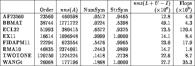
The characteristics of these matrices are given in Table 2.

Table 2: Characteristics of the test matrices. NumSym is the fraction
of nonzeros matched by equal values in symmetric locations.
StrSym is the fraction of nonzeros matched by nonzeros in
symmetric locations.
We distribute the matrix in a two-dimensional block-cyclic fashion.
In this distribution, the P processes (not restricted to be a power of 2)
are arranged as a 2-D process grid of shape  .
The matrix is decomposed into blocks of submatrices. Then, these
blocks are cyclically mapped onto the process grid, in both row and
column dimensions.
Although a 1-D decomposition is more natural to sparse matrices and
is much easier to implement,
a 2-D layout strikes a good balance among locality (by blocking),
load balance (by cyclic mapping), and lower communication volume
(by 2-D mapping). 2-D layouts were used in scalable implementations
of sparse Cholesky factorization [20, 25].
We now describe how we partition a global matrix into blocks.
Our partitioning is based on the notion of unsymmetric supernode
first introduced in [8]. Let L be the lower triangular
matrix in the LU factorization.
A supernode is a range (r:s) of columns of L with
the triangular block just below the diagonal being full,
and with the same row structure below this block.
Because of the identical row structure of a supernode,
it can be stored in a dense format in memory.
This supernode partition is used as our block partition
in both row and column dimensions.
If there are N supernodes in an n-by-n matrix, the matrix
will be partitioned into  blocks of nonuniform size.
The size of each block is matrix dependent.
It should be clear that all the diagonal
blocks are square and full (we store zeros from U in the upper triangle
of the diagonal block), whereas the off-diagonal blocks may be
rectangular and may not be full.
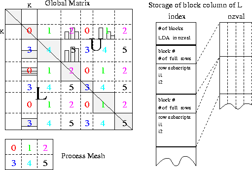
The matrix in Figure 7 illustrates such a partitioning.
By block-cyclic mapping we mean block (I,J) (
  ) is
mapped onto the process at coordinate (I mod
  , J mod
  )
of the process grid.
Using this mapping, a block L(I,J) in the factorization is only needed
by the row of processes that own blocks in row I.
Similarly, a block U(I,J) is only needed
by the column of processes that own blocks in column J.
In this 2-D mapping, each block column of L resides on more than
one process, namely, a column of processes. For example in Figure 7,
the k-th block column of L resides on the column processes {0, 3}.
Process 3 only owns two nonzero blocks, which are not contiguous
in the global matrix.
The schema on the right of Figure 7 depicts the data structure
to store the nonzero blocks on a process.
Besides the numerical values stored in a Fortran-style
array nzval[] in column major order, we need the information to
interpret the location and row subscript of each nonzero. This is stored in
an integer array index[], which includes the
information for the whole block column and for each individual block in it.
Note that many off-diagonal blocks are zero and hence
not stored. Neither do we store the zeros in a nonzero block.
Both lower and upper triangles of the diagonal block are stored in the
L data structure.
A process owns  block columns of L, so it needs
 pairs of index/nzval arrays.
For matrix U, we use a row oriented storage for the block
rows owned by a process, although for the numerical values within each block
we still use column major order. Similarly to L, we also use a pair
of index/nzval arrays to store a block row of U.
Due to asymmetry, each nonzero block in U has the skyline structure
as shown in Figure 7
(see [8] for details on the skyline structure).
Therefore, the organization of the index[] array is different from
that for L, which we omit showing in the figure.
Since we do no dynamic pivoting, the nonzero patterns of L
and U can be determined during symbolic factorization before
numerical factorization begins.
Therefore, the block partitioning and the setup of the data structure
can all be performed in the symbolic algorithm.
This is much cheaper to execute as opposed to
partial pivoting where the size of the data structure cannot be forecast
and must be determined on the fly as factorization proceeds.

Figure 7: The 2-D block-cyclic layout and the data structure
to store a local block column of L.

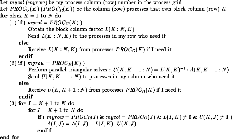
Figure 8: Distributed sparse LU factorization algorithm.
Figure 8 outlines the parallel sparse LU factorization
algorithm. We use Matlab notation for integer ranges and submatrices.
There are three steps in the K-th iteration of
the loop. In step (1), only a column of processes participate in factoring
the block column L(K:N,K). In step (2), only a row of processes participate
in the triangular solves to obtain the block row U(K,K+1:N).
The rank-b update by L(K+1:N,K) and U(K,K+1:N) in step (3) represents
most of the work and
also exhibits more parallelism than the other two steps, where b is the
block size of the K-th block column/row.
For ease of understanding, the algorithm presented here is simplified.
The actual implementation uses a pipelined organization so that
processes  will start step (1) of iteration K+1
as soon as the rank-b update (step (3)) of iteration K to block
column K+1 finishes, before completing the update to the trailing matrix
A(K+1:N, K+2:N) owned by
  .
The pipelining alleviates the lack of parallelism in both steps (1) and (2).
On 64 processors of Cray T3E, for instance, we observed speedups
between 10% to 40% over the non-pipelined implementation.
In each iteration, the major communication steps are send/receive L(K:N,K)
across process rows and send/receive U(K,K+1:N) down process columns.
Our data structure (see Figure 7) ensures that all the blocks of
L(K:N,K) and U(K,K+1:N) on a process
are contiguous in memory, thereby eliminating the need for packing
and unpacking in a send-receive operation or sending many more smaller
messages. In each send-receive pair, two messages are exchanged, one
for index[] and another for nzval[].
To further reduce the amount of communication, we employ the
notion of elimination dags (EDAGs) [18].
That is, we send the K-th column of L rowwise
to the process owning the J-th column of L only if
there exists a path between (super)nodes K and J in the elimination dags.
This is done similarly for the columnwise communication of rows of U.
Therefore, each block in L may be sent to fewer than  processes
and each block in U may be sent to fewer than
  processes.
In other words, our communication takes into account the sparsity of the
factors as opposed to ``send-to-all'' approach in a dense factorization.
For example, for AF23560 on 32 (
  ) processes,
the total number of messages is reduced from 351052 to 302570, or
16% fewer messages. The reduction is even more with more processes or
sparser problems.

Figure 9: Distributed lower triangular solve  .
.
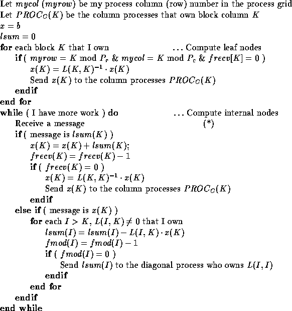
The sparse lower and upper triangular solves are also designed around
the same distributed data structure.
The forward substitution proceeds from the
bottom of the elimination tree to the root,
whereas the back substitution proceeds from the root to the bottom.
Figure 9 outlines the algorithm for sparse lower
triangular solve.
The algorithm is based on a sequential variant called
``inner product'' formulation.
In this formulation, before the K-th subvector x(K) is solved,
the update from the inner product of L(K,1:K-1) and x(1:K-1)
must be accumulated and subtracted from b(K).
The diagonal process, at the coordinate (K mod  , K mod
  ) of
the process grid, is responsible for solving x(K).
Two counters, frecv and fmod, are used to facilitate the asynchronous
execution of different operations. frecv[K] counts the number of process
updates to x(K) to be received by the diagonal process owning x(K).
This is needed because L(K,1:K-1) is distributed among
the row processes
  ,
and due to sparsity, not all processes in
  contribute
to the update. When frecv(K) becomes zero, all the necessary updates
to x(K) are complete and x(K) is solved.
fmod(K) counts the number of block modifications to be summed
into the local inner product update (stored in lsum(K)) to x(K).
When fmod(K) becomes zero, the partial sum lsum(K) is sent to
the diagonal process that owns x(K).
The execution of the program is message-driven.
A process may receive two types of messages, one is the partial sum lsum(K),
another is the solution subvector x(K). Appropriate action is taken
according to the message type.
The asynchronous communication enables large overlapping between
communication and computation. This is very important because
the communication to computation ratio is much higher
in triangular solve than in factorization.
The algorithm for the upper triangular solve is similar to that
illustrated in Figure 9. However, because of the row oriented
storage scheme used for matrix U, there is a slight complication in
the actual implementation. Namely, we have to build two vertical linked
lists to enable rapid access of the matrix entries in a block column of U.
Recall that we partition the blocks based on supernodes,
so the largest block size equals the number of columns of the largest
supernode. For large matrices, this can be a few thousand, especially
towards the end of matrix L. Such a large granularity would lead to very
poor parallelism and load balance. Therefore, when this occurs,
we break the large supernode into smaller chunks, so that each chunk
does not exceed our preset threshold, the maximum block size.
By experimenting, we found that a maximum block size between
20 and 30 is good on the Cray T3E. We used 24 for all the performance
results reported in this section.

Table 3: LU factorization time in seconds and Megaflop rate on the 512 node
T3E-900.
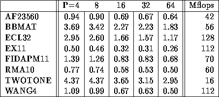
Table 3 shows the performance of the factorization
on the Cray T3E-900. The symbolic analysis (steps (1) and (2)
in Figure 1) is not yet parallel,
so we start with a copy of the entire matrix on each
processor, and run steps (1) and (2) independently on each processor.
Thus the time is independent of the number of processors.
The first column of Table 3 reports the time spent in the
symbolic analysis. The memory requirement of the symbolic
analysis is small, because we only store and manipulate the
supernodal graph of L and the skeleton graph of U,
which are much smaller than the graphs of L and U.
The subsequent columns in the table show the factorization time
with a varying number of processors. For four large matrices
(BBMAT, ECL32, FIDAPM11 and WANG4), the factorization
time continues decreasing up to 512 processors, demonstrating good scalability.
The last column reports the numeric factorization rate in Mflops.
More than 8 Gflops is achieved for matrix ECL32.
This is the fastest published result we have seen
for any implementation of parallel sparse Gaussian elimination.
Table 3 starts with P=4 processors because some of the
examples could not run with fewer processors.
As a reference, we compare our distributed memory code to our
shared memory SuperLU_MT code using small numbers of processors.
For example, using 4 processor DEC AlphaServer 8400 (SMP)
 , the factorization
times of SuperLU_MT for matrices AF23560 and EX11 are 19 and 23 seconds,
respectively, comparable to the 4 processor T3E timings.
This indicates that our distributed data structure and message passing
algorithm do not incur much overhead.
Table 4 shows the performance of the lower and upper
triangular solves altogether.
When the number of processors continues increasing beyond 64,
the solve time remains roughly the same.
Although triangular solves do not achieve high Megaflop rates,
the time is usually much less than that for factorization.

Table 4: Triangular solves time in seconds and Megaflop rate on the T3E-900.
The efficiency of a parallel algorithm depends mainly on how the workload
is distributed and how much time is spent in communication.
One way to measure load balance is as follows.
Let  denote the number of floating-point operations performed
on process i. We compute the load balance factor
 .
In other words, B is the average workload divided by the maximum
workload. It is clear that
  , and higher B indicates
better load balance. The parallel runtime is at least the runtime
of the slowest process, whose workload is highest.
In Table 5 we present the load balance factor B for both
factorization and solve phases.
As can be seen from the table, the distribution of workload is
good for most matrices, except for TWOTONE.
In the same table, we also show the fraction of the runtime spent
in communication. The numbers were collected from the performance
analysis tool called Apprentice on the T3E.
The amount of communication is quite excessive.
Even for the matrices that scale well, such as BBMAT, ECL32,
FIDAPM11 and WANG4, more than 50% of the factorization time is spent in
communication. For the solve, which has much smaller amount of computation,
communication takes more than 95% of the total time.
We expect the percentage of communication will be even higher with
more processors, because the total amount of computation is more or
less constant.

Table 5: Load balance and communication on 64 processors Cray T3E.
Although TWOTONE is a relatively large matrix, the factorization
does not scale as well as for the other large matrices.
One reason is that the present submatrix
to process mapping results in very poor load distribution.
Another reason is due to long time in communication.
When we look further
into communication time using Apprentice, we found that
processes are idle 60% of the time waiting to receive the
column block of L sent from a process column on the left
(step (1) in Figure 8), and are idle 23% of the time waiting
to receive the row block of U sent from a process row from above
(step (2) in Figure 8). Clearly, the critical path of the
algorithm is in step (1), which must preserve certain precedence relation
between iterations. Our pipelining method shortens the critical path
to some extent, but we expect the length of the critical path can be further
reduced by a more sophisticated DAG (task graph) scheduling.
For the solve, we found that processes are idle 73% of the time waiting
for a message to arrive (at line (*) in Figure 9).
So on each process there is not much work to do but a large amount
of communication.
These communication bottlenecks also occur for the other matrices,
but the problems are not so pronounced as TWOTONE.
Another problem with TWOTONE is that supernode size
(or block size) is very small, only 2.4 columns on average.
This results in poor uniprocessor performance and low Megaflop rate.
We propose a number of techniques in place of partial pivoting
to stabilize sparse Gaussian elimination. Their effectiveness
is demonstrated by numerical experiments.
These techniques enable static analysis of the nonzero structure
of the factors and the communication pattern. As a result, a more
scalable implementation becomes feasible on large-scale distributed memory
machines with hundreds of processors.
Our preliminary software is being used in a
quantum chemistry application at Lawrence Berkeley National Laboratory,
where a complex unsymmetric system of order 200,000 has been solved
within 2 minutes.
Although the current GESP algorithm is successful for a large number of
matrices, it fails to solve one finite element matrix, AV41092,
because the pivot growth is still too large with any combination
of the current techniques.
We plan to investigate other complementary techniques to further
stabilize the algorithm.
For example, we can use a judicious amount of extra precision to
store some matrix entries more accurately, and to perform internal
computations more accurately. This facility is available for free on Intel
architectures, which performs all arithmetic most efficiently
in 80-bit registers, and at modest cost on other machines.
The extra precision can be used in both factorization and residual
computation.
We can also mix static and partial pivoting by only pivoting within a
diagonal block owned by a single processor (or SMP within a cluster
of SMPs). This can further enhance stability.
We can use a more aggressive pivot size control strategy in step (4)
of the algorithm. That is, instead of setting tiny pivots to
 , we may set it to the largest
magnitude of the current column. This incurs a non-trivial
amount of rank-1 perturbation to the original matrix. In the
end, we use Sherman-Morrison-Woodbury formula [7]
to recover the inverse of the original matrix, at the cost
of a few more steps of inverse iteration.
It remains to be seen in what circumstances
these ideas should be employed in practice. There are also theoretical
questions to be answered.
In order to make the solver entirely scalable, we need to parallelize
the symbolic algorithm. In this case, we will start with
the matrix initially distributed in some manner.
The symbolic algorithm then determines the best layout for
the numeric algorithms, and redistributes matrix if necessary.
This also requires us to provide a good interface so the user
knows how to input the matrix in the distributed manner.
For the LU factorization, we will investigate more general functions
for matrix-to-process mapping and scheduling of computation and communication
by exploiting more knowledge from the EDAGs. This is expected
to relax much of the synchrony in the current factorization algorithm,
and reduce communication.
We also consider switching to a dense factorization, such as the one
implemented in ScaLAPACK [4], when
the submatrix at the lower right corner becomes sufficiently dense.
The uniprocessor performance can also be improved by amalgamating
small supernodes into large ones.
To speed up the sparse triangular solve, we may apply some graph
coloring heuristic to reduce the number of parallel
steps [21].
There are also alternative algorithms other than substitutions,
such as those based on partitioned inversion [1]
or selective inversion [24].
However, these algorithms usually require preprocessing or different matrix
distributions than the one used in our factorization. It is unclear
whether the preprocessing and redistribution will offset the benefit
offered by these algorithms, and will probably depend on the number
of right-hand sides.
Duff and Koster [13] applied the techniques of permuting
large entries to the diagonal in both direct and iterative methods.
In their direct method using a multifrontal approach, the numeric
factorization first proceeds with diagonal pivots as previously chosen
by the analysis on the structure of  . If a diagonal entry is
not numerically stable, its elimination will be delayed,
and a larger frontal matrix will be passed to the later stage.
They showed that using the initial permutation, the
number of delayed pivots were greatly reduced in factorization.
They experimented with some iterative methods such as GMRES, BiCGSTAB and
QMR using ILU preconditioners. The convergence rate is substantially
improved in many cases when the initial permutation is employed.
Amestoy, Duff and L'Excellent [2] implemented
the above multifrontal approach for distributed memory machines.
The host performs the fill-reducing ordering, estimates each frontal
matrix structure, and statically maps the assembly tree, all
based on the symmetric pattern of  , and then sends the information
to the other processors. During numerical factorization, each frontal
matrix is factorized by a master processor and one or more
slave processors. Due to possible delayed pivots, the frontal
matrix size may be different than predicted by the analysis phase.
So the master processor dynamically determines how many slave processors
will be actually used for each frontal matrix.
They showed good performance on 32 processors IBM SP2.
MCSPARSE [16] is a parallel unsymmetric linear system solver.
The key component in the solver is the reordering step, which transforms
the matrix into a bordered block upper triangular form.
Their reordering first uses an unsymmetric ordering to put relatively
large entries on the diagonal. The algorithm is a modified version of
Duff [11, 12]. After this unsymmetric ordering, they
use several symmetric permutations, which preserve the diagonal, to
order the matrix into the desired form.
With large diagonal entries, there is a better chance of obtaining
a stable factorization by pivoting only within the diagonal blocks.
The number of pivots from the border is thus reduced.
Large and medium grain parallelism is then exploited to factor the
diagonal blocks and eliminate the bordered blocks.
They implemented the parallel factorization algorithm on a
32 processor Cedar, an experimental shared memory machine.
Fu, Jiao and Yang [15] designed a parallel LU factorization
algorithm based on the following static information. The sparsity
pattern of the Householder QR factorization of A contains
the union of all sparsity patterns of the LU factors of A
for all possible pivot selections. This has been used
to do both memory allocation and computation conservatively
(on possibly zero entries), but it can be arbitrarily conservative,
particularly for matrices arising from circuit and device simulations.
For several matrices that do not incur much overestimation, they
showed good factorization speed on 128 processors Cray T3E.
It will be interesting to compare the performance of the
different approaches.
We are grateful to Iain Duff for giving us access to the early version
of the Harwell subroutine MC64, which permutes large entries
to the diagonal.
References
- 1
-
Fernando L. Alvarado, Alex Pothen, and Robert Schreiber.
Highly parallel sparse triangular solution.
In Alan George, John R. Gilbert, and Joseph W.H. Liu, editors,
Graph theory and sparse matrix computation, pages 159-190. Springer-Verlag,
New York, 1993.
- 2
-
P. R. Amestoy, I. S. Duff, and J.-Y. L'Excellent.
Multifrontal parallel distributed symmetric and unsymmetric solvers.
Technical Report RAL-TR-98-051, Rutherford Appleton Laboratory, 1998.
- 3
-
E. Anderson, Z. Bai, C. Bischof, J. Demmel, J. Dongarra, J. Du Croz,
A. Greenbaum, S. Hammarling, A. McKenney, S. Ostrouchov, and D. Sorensen.
LAPACK Users' Guide, Release 2.0.
SIAM, Philadelphia, 1995.
324 pages.
- 4
-
L. S. Blackford, J. Choi, E. D'Azevedo, J. Demmel, I. Dhillon, J. Dongarra,
S. Hammarling, G. Henry, A. Petitet, K. Stanley, D. Walker, and R. C. Whaley.
ScaLAPACK Users' Guide.
SIAM, Philadelphia, 1997.
325 pages.
- 5
-
Timothy A. Davis.
University of Florida sparse matrix collection.
http://www.cise.ufl.edu/
 davis.
- 6
-
Timothy A. Davis, John R. Gilbert, Esmond Ng, and Barry Peyton.
Approximate minimum degree ordering for unsymmetric matrices.
Talk presented at XIII Householder Symposium on Numerical Algebra,
June 1996. Journal version in preparation.
- 7
-
James W. Demmel.
Applied Numerical Linear Algebra.
SIAM, Philadelphia, 1997.
- 8
-
James W. Demmel, Stanley C. Eisenstat, John R. Gilbert, Xiaoye S. Li, and
Joseph W.H. Liu.
A supernodal approach to sparse partial pivoting.
Technical Report UCB//CSD-95-883, Computer Science Division, U.C.
Berkeley, 1995.
To appear in SIAM J. Matrix Anal. Appl.
- 9
-
James W. Demmel, John R. Gilbert, and Xiaoye S. Li.
An asynchronous parallel supernodal algorithm for sparse gaussian
elimination.
Technical Report UCB//CSD-97-943, Computer Science Division, U.C.
Berkeley, 1997.
To appear in SIAM J. Matrix Anal. Appl.
- 10
-
James W. Demmel, John R. Gilbert, and Xiaoye S. Li.
SuperLU and SuperLU_MT, November 1997.
http://www.netlib.org/scalapack/prototype/.
- 11
-
I. S. Duff.
Algorithm 575. Permutations for a zero-free diagonal.
ACM Trans. Mathematical Software, 7:387-390, 1981.
- 12
-
I. S. Duff.
On algorithms for obtaining a maximum transversal.
ACM Trans. Mathematical Software, 7:315-330, 1981.
- 13
-
Iain S. Duff and Jacko Koster.
The design and use of algorithms for permuting large entries to the
diagonal of sparse matrices.
Technical Report RAL-TR-97-059, Rutherford Appleton Laboratory, 1997.
- 14
-
I.S. Duff, R.G. Grimes, and J.G. Lewis.
Users' guide for the Harwell-Boeing sparse matrix collection
(release 1).
Technical Report RAL-92-086, Rutherford Appleton Laboratory, December
1992.
- 15
-
C. Fu, X. Jiao, and T. Yang.
Efficient sparse LU factorization with partial pivoting on
distributed memory architectures.
IEEE Trans. Parallel and Distributed Systems, 9(2):109-125,
1998.
- 16
-
K. A. Gallivan, B. A. Marsolf, and H. A. G. Wijshoff.
Solving large nonsymmetric sparse linear systems using MCSPARSE.
Parallel Computing, 22:1291-1333, 1996.
- 17
-
J. George.
Nested dissection of a regular finite element mesh.
SIAM J. Numerical Analysis, 10:345-363, 1973.
- 18
-
John R. Gilbert and Joseph W.H. Liu.
Elimination structures for unsymmetric sparse LU factors.
SIAM J. Matrix Anal. Appl., 14(2):334-352, April 1993.
- 19
-
G. Golub and C. Van Loan.
Matrix Computations.
Johns Hopkins University Press, Baltimore, MD, Third edition, 1996.
- 20
-
A. Gupta and V. Kumar.
Optimally scalable parallel sparse cholesky factorization.
In The 7th SIAM Conference on Parallel Processing for Scientific
Computing, pages 442-447, 1995.
- 21
-
Mark T. Jones and Paul E. Plassmann.
Scalable iterative solution of sparse linear systems.
Parallel Computing, (20):753-773, 1994.
- 22
-
Xiaoye S. Li.
Sparse Gaussian elimination on high performance computers.
Technical Report UCB//CSD-96-919, Computer Science Division, U.C.
Berkeley, September 1996.
Ph.D dissertation.
- 23
-
Joseph W.H. Liu.
Modification of the minimum degree algorithm by multiple elimination.
ACM Trans. Math. Software, 11:141-153, 1985.
- 24
-
Padma Raghavan.
Efficient parallel sparse triangular solution with selective
inversion.
Technical Report CS-95-314, Department of Computer Science,
University of Tennessee, 1995.
- 25
-
E. E. Rothberg and A. Gupta.
An efficient block-oriented approach to parallel sparse cholesky
factorization.
In Supercomputing, pages 503-512, November 1993.
- 26
-
Message Passing Interface (MPI) forum.
http://www.mpi-forum.org/.
Xiaoye Li
is a research staff at NERSC, the National Energy
Scientific Computing Center at Lawrence Berkeley National Laboratory,
Her main research interests are in parallel computing and sparse linear
algebra.
She received her Ph.D. in Computer Science from UC Berkeley in 1996.
Her thesis research was developing efficient algorithms and software
for solving large sparse linear systems on high performance architectures.
This research resulted in SuperLU library, one of the fastest
implementations of parallel sparse Gaussian elimination
available to the public.
James Demmel
is a professor of Computer Science and Mathematics
at the University of California at Berkeley. His research is
in high performance computing and numerical linear algebra.
He is co-principal investigator on the LAPACK and ScaLAPACK
projects, which are leading numerical libraries for high
performance machines. He was an NSF-CBMS Lecturer on
Parallel Numerical Linear Algebra in 1995.
Recent awards include SIAM's J. H. Wilkinson Prize
in Numerical Analysis and Scientific Computing in 1993,
and two SIAM SIAG prizes for best papers in linear algebra.
 .
However partial pivoting is not the only way to control element growth;
there are a variety of alternative techniques.
In this section we present these alternatives, and
show by experiments that appropriate combinations of them
can effectively stabilize Gaussian elimination.
Furthermore, these techniques are usually inexpensive compared
to the overall solution cost, especially for large problems.
